Classification of Asymmetric Proximity Data - Semantic Scholar

Journal of Classification DOI: 10.1007/s00357- 014- 9159-6

Classification of Asymmetric Proximity Data Donatella Vicari Sapienza University of Rome, Italy

Abstract: When clustering asymmetric proximity data, only the average amounts are often considered by assuming that the asymmetry is due to noise. But when the asymmetry is structural, as typically may happen for exchange flows, migration data or confusion data, this may strongly affect the search for the groups because the directions of the exchanges are ignored and not integrated in the clustering process. The clustering model proposed here relies on the decomposition of the asymmetric dissimilarity matrix into symmetric and skew-symmetric effects both decomposed in within and between cluster effects. The classification structures used here are generally based on two different partitions of the objects fitted to the symmetric and the skew-symmetric part of the data, respectively; the restricted case is also presented where the partition fits jointly both of them allowing for clusters of objects similar with respect to the average amounts and directions of the data. Parsimonious models are presented which allow for effective and simple graphical representations of the results. Keywords: Asymmetric dissimilarities; Partition; Skew-Symmetric matrix; LeastSquares.

1. Introduction and Background The large majority of classification models are typically applied to square symmetric proximity matrices between objects such as the most common hierarchical clustering methods. However, in several applications data are intrinsically asymmetric as it frequently happens in case of preferences (sociomatrices), exchanges (e.g. import-export, brand switching), migration data, and confusion data. ____________ Author’s Address: D. Vicari, Dipartimento di Scienze Statistiche, Sapienza University of Rome, pl. A. Moro 5, 00185, Rome, Italy, e-mail: [email protected].

D. Vicari

Such data are often dealt with by ignoring the asymmetry and considering only the lower (upper) triangular part of the square matrix or by averaging the two different values related to each pair of objects. In this way the asymmetric component of the data is assumed due to random error or noise. However, when the asymmetry is assumed to be structural and/or it is prominent, such approaches may eliminate a significant asymmetric effect which may embody some important information of a systematic nature: then the asymmetry is of interest in its own right. In multidimensional scaling framework (Borg and Groenen 2005), different approaches model the asymmetry itself to account for not only the average amount but even the direction of the data, which can be relevant especially in particular contexts, such as for example for migration data or exchanges between countries or confusion rates between stimuli. To represent in low-dimensional spaces jointly the symmetry and the skew-symmetry of the data, several models have been proposed (for example, Escoufier and Grorud 1980; Zielman and Heiser 1996; Rocci and Bove 2002; see also Borg and Groenen 2005). In the classification context such kind of data have been considered in several papers in different fields of research (an extensive review is considered in Chapter 5 of the book on Data Analysis of Asymmetric Structures by Saito and Yadohisa 2005). Cluster analysis methodologies for asymmetric data have been developed under two major approaches. In one approach, the asymmetric proximities are regarded as a special case of two-mode two-way data, where the rows and the columns are considered two different modes. A class of algorithms following this approach generally aims at fitting tree structures, that is, ultrametric and/or additive trees to the data (Furnas 1980; DeSarbo and De Soete 1984; DeSarbo, Manrai, and Burke 1990; De Soete, DeSarbo, Furnas, and Carroll 1984), allowing also for the graphical representations of the asymmetric clustering by generalized dendrograms. Another class of methods is based on reordering of rows and columns of the data to find the clusters (McCormick, Schweitzer, and White 1972; Arabie, Schleutermann, Daws, and Hubert 1988; Eckes and Orlik 1993). A generalization of ADCLUS by Shepard and Arabie (1979) for the case of asymmetric or two-mode data has been also proposed by DeSarbo (1982) and by Both and Gaul (1986). In the other approach, asymmetric proximity data are treated in accordance with the original form of the data, that is, one-mode two-way data, and analyzed in view of the asymmetry. The algorithms proposed are generally extensions of the classical agglomerative hierarchical algorithms such as single, complete and average linkage for asymmetric data (Hubert 1973; Fujiwara 1980; Okada

Classification of Asymmetric Proximity Data

and Iwamoto 1996); updating formulas to generalize asymmetric hierarchical clustering algorithms have been proposed in a comprehensive unified framework (Yadohisa 2002; Takeuchi, Saito, and Yodhisa 2007), providing also the representation of the clustering results by asymmetric dendrograms. Ozawa (1983) developed a hierarchical clustering algorithm, called CLASSIC, by using the nearest neighbors relation. Within the same one-mode framework and following the same approach used for scaling an asymmetric matrix (Gower 1977, Constantine and Gower 1978) which relies essentially on the canonical decomposition of the skew symmetric matrix, Brossier (1982) has considered the approximation of an asymmetric dissimilarity matrix by two orthogonal matrices: an ultrametric one by a hierarchical classification of the objects, fitting the symmetric part of the data (the average amount) and a skew symmetric matrix representing the surplus/deficit of the dissimilarities between objects. The novelty of the model by Brossier (1982) is that the asymmetry of the data is explicitly taken into account in terms of symmetric and skew-symmetric effects, but the hierarchical classification fits only the symmetric part (i.e. the average amounts), while the directions of the data are not involved in any clustering process. In the same framework, since any skew-symmetric matrix can itself be interpreted as containing two separate sources of information (the directionality of the dominance relationship given by the signs and the absolute magnitude of the dominance given by the absolute value), an extension of the notion of order constrained matrix (specifically, antiRobinson form) appropriate for a symmetric proximity matrix is adopted also for the skew-symmetric part. In such a way, that the degree of dominance is perfectly depicted by having an anti-Robinson form (optimal reordering of the objects) and the direction of the dominance is depicted in the reordered matrix of the signs (Hubert, Arabie, and Meulman 2001). The model proposed here is framed in the same one-mode approach and considers simultaneously rows and columns of a dissimilarity matrix to explicitly account for both the symmetry and the skew-symmetry of the data when fitting the classification of the objects, so that the average amounts and the directions are jointly involved in the clustering process. Specifically, the clustering model relies on the decomposition of the asymmetric dissimilarity matrix into symmetric and skew-symmetric effects both decomposed in within and between cluster effects. The paper is structured as follows. The reasoning motivating the methodology is introduced in the next section through simple illustrative examples. After providing the essential notation, in Section 3 the classification model for asymmetric data is formalized and in Section 4 an appropriate Alternating Least Squares algorithm is provided to fit the

D. Vicari

model. The results of a simulation study in Section 5 and two applications to real data in Section 6 illustrate the performance of the algorithm, the potentiality of the method and the possible graphical display of the results. Finally, some concluding remarks and future developments and enhancements are presented in Section 7. 2. Motivating Example Clusters based only on the symmetric part of the data consist of objects having quite high similarities (they are closer than objects in different clusters), i.e. they share high average amounts. The question is: where are such amounts directed? To give a flavour of the reasoning motivating the methodology, we consider some illustrative examples of different asymmetric structures and the clustering results we may have (the details of the clustering methodology fitted in such examples will be formalized in the following Sections). Figures 1(a) and (c) display two situations where the locations of the dots account for the symmetric dissimilarities between six objects and the arrows show the directions of the exchanges: the locations of the objects exhibit triangular shape configurations, but the tendency of asymmetry looks quite different. They both reveal that two objects (B and D) direct equally towards two out of the remaining four objects within the same triangular (clustering) structure, but the between asymmetry differs. In the first case a solid arrow from the first triplet towards the second one is present, meaning that all objects in cluster (A,B,C) point equally towards the other triplet (D,E,F) with asymmetries of equal strengths. In the second case (Figure 1(c)), the two dotted lines indicate that only object B in cluster 1 directs towards all the objects in cluster 2 and, conversely, only object D in the second cluster receives from the first triplet. For the sake of clarity, in the figures all the arrowed lines correspond to skew-symmetry values equal to 0.5 and 1, respectively. In Figure 1(e) an additional object G is located slightly closer to the second triplet than the first one and receives only from B while it directs only to D. Case 1 In the first situation (Figure 1(a)), two distinct clusters are evident with respect to both the locations of the dots and the directions of the exchanges: (A,B,C) is an out-cluster and (D,E,F) is an in-cluster. Even if the degree of asymmetry is relatively low because the skew-symmetric component accounts for the 4.95% of the total dissimilarities, such asymmetry reveals a pattern present both within and between clusters.


Figure 1. Illustrative examples of asymmetric data: solid arrows indicate that all objects in one cluster point equally to the other cluster; dotted arrows indicate that only one object in a cluster directs to (receives from) the objects in the other cluster.

When clustering the objects separately from either the symmetric or the skew-symmetric component or simultaneously from the original asymmetric dissimilarities, the common partition into two groups is found: it accounts for the 98.45% of the symmetric part of the data and perfectly fits

D. Vicari

the skew-symmetric component. The tree in Figure 1(b) displays the two groups where the within asymmetry is represented by the vertical dashed branches below/above the zero line, indicating which objects move from/to the others within each cluster. The between asymmetry is displayed by the shifted cluster heights below/above the horizontal dotted line to indicate the between cluster asymmetries. From the tree is evident that all objects in the first cluster (A,B,C) move towards the objects in the second one (D,E,F), while within each cluster only one object originates towards the remaining two ones. Case 2 In the situation of Figure 1(c), the pattern of the between asymmetry is not fully complete and the degree of asymmetry is quite low (the skewsymmetries account for the 3.03% of the total variation), but it is still systematic and cluster related. When the objects are clustered with respect to only the object locations, the partition into clusters (A,B,C) and (D,E,F) fits well the symmetrized dissimilarities as in case 1. Conversely, when we search for a partition of objects which best fits the average directions of the exchanges regardless the average amounts, we get different groups (A,B,C,D) and (E,F) where out-objects and in-objects are clustered, respectively, accounting for the 87.73% of the skew-symmetrized dissimilarities. The tree in Figure 1(d) displays the partition into clusters (A,B,C) and (D,E,F) which best fits simultaneously both the symmetric and the skew-symmetric dissimilarities. In addition to the average between asymmetry displayed by the shifts below/above the horizontal dotted line (average within amount level), the between asymmetry due to each object is represented by a vertical dotted segment. It is evident that even if the whole first cluster move towards the other, the main contribution to such a between skew-symmetry is due to object B. The same considerations hold for object D which is the main destination of the second cluster: in such a case, cluster (A,B,C) may be still regarded as an out-cluster directed towards (D,E,F). The within asymmetry is perfectly accounted for by the

ˆ approximates partition as in Case 1 and the fitted dissimilarity matrix D well the original D in terms of relative Residual Sum of Squares (RSS=0.0195). In Case 1 the symmetric and skew-symmetric parts of the data share naturally the same common partition and clustering the objects from the two components, either separately or jointly, gives the same results in terms of groups and goodness of fit. In Case 2 the two separate clusterings give different partitions: the first one reflects the proximity of the objects in terms of average amounts (dot locations) and the second one reflects the directionality and the magnitude of the dominance relationship between


objects. In such a respect (A,B,C,D) are mainly origins of the exchanges and (E,F) are just destinations. Clearly, separately clustering the symmetries and the skew-symmetries approximates the original dissimilarities (RSS=0.0188 vs RSS=0.0195) slightly better, but fitting a single partition of the objects allows for a better understanding of the exchanges with only a small loss of the fit. Case 3 In situation of Figure 1(e), the degree of asymmetry is the same as before (the skew-symmetries account for the 3.04% of the total variation). As evident from the dot locations, when the objects are clustered from the symmetrized dissimilarities, the partition into clusters (A,B,C) and (D,E,F,G) is found which accounts for the 95.2% of the symmetric part. Conversely, when we search for a partition of the objects from the skewsymmetries, we get the groups (A,C,D,G) and (B,E,F) accounting for the 78.47% of the skew-symmetrized dissimilarities. The two partitions identify two different clustering structures which together approximate the original dissimilarity matrix (RSS=0.101) reasonably well. The tree in Figure 1(f), which represents the partition into clusters (A,B,C,G) and (D,E,F) obtained when a single partition is required, shows a situation very similar to the one of Figure 1(d), where evidently object G exhibits the same behaviour of the objects in its cluster, clearly with a higher average within dissimilarity than Case 2. The Residual Sum of Squares (RSS=0.102) for such a restricted solution is nearly the same, but the partition allows for the identification of cohesive groups which reflect common behaviours in terms of average amounts of the exchanges and directionality of the dominance relationships. 2.1 Clusters of Asymmetric Data We need to better clarify the meaning of the clusters of objects obtained from the skew-symmetric part of the data as illustrated above. When clustering from the skew-symmetric part of the data, regardless the average proximity, objects belonging to the same group: a) share the same behaviours in terms of exchanges directed towards the other clusters, i.e. some clusters are mainly origins towards (destinations from) some other clusters; b) form closed systems of internal exchanges. For example, clusters may identify weak vs strong brands in the context of brand switching data, exporting vs importing countries, groups of social actors having the same interactions with other social groups. In some cases the presence of a strong imbalance between (groups of) objects may be interesting when a strong average amount is also

D. Vicari

present and the meaning of the clusters derived from the imbalances need to be analyzed by integrating the information from the average amounts. In such a respect, a unique partition may be more useful and interpretable than the two independent ones (from the symmetric and the skewsymmetric part of the data). As suggested by a referee, for most types of flow data these same clusters are difficult to find in the partitions obtained by the symmetric part of the data, where usually origins and destinations are found together in the same clusters (e.g., import/export data). This makes it difficult to find a "good" common partition in these situations, and may be in general even harder for highly skew-symmetric data. By contrast, when such a common partition is a good compromise (in terms of a loss function) between the two partitions from the symmetric and skew-symmetric data, the clusters include objects having both the same average amounts (close or similar objects) and the same average imbalances (in terms of intensity and direction) directed to the other clusters. However, when the fit is not as good as we expect we conclude that a common clustering pattern underlying the asymmetries does not exist. Moreover, the decomposition of the asymmetries into between and within effects results in clusters having similar exchanges between objects within the same cluster, given the average amounts (for example, exchanges between leader market brands or countries, or between social actors with large relations), while exchanges between clusters refer to objects with generally different average symmetries. Note that the symmetric part of the data is generally prominent in real applications and because of the non-negativity of the asymmetric dissimilarities, the imbalances are bounded so that strong imbalances generally correspond to large amounts between objects. 3. The Model Let D=[dij] be an (nn) two-way one-mode matrix of pairwise proximities measured on a set of n objects, where dij is not necessarily equal to dji. Without loss of generality we suppose that D is a dissimilarity matrix, dij is non-negative (we may always add a constant to the whole matrix and obtain non-negative dissimilarities) and dij=0 means that no dissimilarity exists between objects i and j. Generally, the model proposed detects optimal partitions of the objects with respect to both rows and columns of the asymmetric dissimilarity matrix, respectively, i.e. the oriented dissimilarities between objects. Let us recall that any square matrix D can be uniquely decomposed into a sum of a symmetric matrix S and a skew-symmetric matrix K


D  S  K  (D  D) / 2  (D  D) / 2 ,

(1)

where S and K are orthogonal to each other, i.e. trace(SK)  0 . The element sij of S represents the average amount between objects i and j and the element kij of K represents the disequilibrium between i and j i.e. the amount by which dij differs from the mean sij. Because of the orthogonality of S and K, it is possible to measure how the two components of the dissimilarities weigh differently: ||S||2/||D||2 and ||K||2/||D||2 are the parts of the total variability accounted for by the symmetric and skew-symmetric component of the data, respectively; the latter measures the degree of asymmetry of the data and may be not ignorable. When the asymmetry is supposed to be structural (systematic) and/or the degree of asymmetry is prominent, we may suppose that it may affect the classification of the objects. Therefore, we assume that the two orthogonal parts of the dissimilarity data, namely S and K, should be approximated by different classification structures generally depending on different partitions of the objects; as a special case they may share the same common partition of the objects. A general model may be defined for partitioning the asymmetric matrix D into symmetric and skew-symmetric effects where both are decomposed into within and between cluster effects. Actually, it gives rise to a class of models that differ whether or not a clustering term for either the symmetric or the skew-symmetric component is included: for example, we may be interested in clustering the objects only from the skew-symmetric dissimilarities, while for the symmetric part a form of MDS could also be useful. Conversely, a clustering for modelling the symmetry can be searched and the asymmetry may be incorporated to represent the directions of the dissimilarities regardless the presence of a partition of the objects. Hence, a series of models may be formulated with a common general structure including variations whether or not the (same or different) clustering for modelling symmetry and skew-symmetry is present:

D

S  K   P    

PW  P B

ES

M    

EK

MW  M B

 (PW  MW )  (PB  M B )  E ,

(2)

where the general error term E represents the part of D not accounted for by the model.

D. Vicari

According to the different specifications of the structures approximating S and K, a series of models originate and some terms in the righthand side in (2) may be missing. Specifically, a)

When only the symmetric part of the data S is clustered by a hierarchical or non-hierarchical model (for example clustering structures as in Hubert, Arabie, and Meulman, 2006 or Vichi, 2008), the objects are assumed to be homogeneous in terms of skew-symmetry and the between term MB is null: D=(PW+ MW) + PB +E. Here the between effect is due only to the partition from the symmetric amounts and the model K= MW+ EK can be a representation of the average directions of the dissimilarities (for example, for a review of models to represent the skewsymmetry see Chapter 3 of the book on Data Analysis of Asymmetric Structures by Saito and Yadohisa 2005).

b)

When only the skew-symmetric component of D is clustered, the objects are assumed to belong to one cluster approximating the symmetric matrix S and only the within term PW is present in (2): D= PW+(MB+MW)+E. The model approximating the symmetric matrix S can be also a form of symmetric MDS useful to represent the data.

c)

When the objects are clustered from both S and K, the within and between effects generally depend on two independent partitions specified by two membership matrices US and UK, fitted on the symmetric and the skew-symmetric component, respectively: D= [PW(US) + PB(US)] + [MB(UK) + MW(UK)] + E.

d)

A restricted model relies on the assumption that both the clustering structures approximating S and K depend on a unique partition and, consequently, US =UK =U: D= [PW(U) + PB(U)] + [MB(U) + MW(U)] + E. In this case the common partition consists of clusters of objects similar with respect to the average amounts and the directions of the exchanges.

In the following, we focus on case c) and its special case d) by assuming that the symmetric matrix S is approximated by a dissimilarity matrix P representing a clustering structure based on a partition of the objects, while K is approximated by a skew symmetric matrix M also depending on a partition of the objects, which may be generally different. Without loss of generality we consider here some kinds of classification structures P approximating S and, when another specification for P is assumed, the model can be extended straightforwardly.


3.1 Clustering Structure Approximating the Symmetric Component S We assume that the symmetric matrix S is approximated by a classification matrix P defining a partition of objects where the c clusters may have different heterogeneities (lack of cohesion within clusters) and isolations between clusters (Vichi 2008). The classification matrix P is a dissimilarity matrix specifying the clustering structure and may generally satisfy some further order constraints on the triplets of its entries, in order to define a specific clustering model, e.g., partition, covering, hierarchy (Hubert et al. 2006; Vichi 2008). Specifically, we consider here a partition of the n objects into c disjoint clusters uniquely identified by an (nc) binary membership matrix U=[uit] specifying for each object i whether it belongs to cluster t (t=1,…,c) or not, i.e., uit=1 if i belongs to t, uit = 0 otherwise. Matrix P can be decomposed into the within and between components depending on U

P  PW  PB   UDW U  diag (UDW U)  UDBU,

(3)

W

where DW  [dkk ] is a (cc) diagonal matrix whose diagonal entries B

represent the c cluster-specific heterogeneities and DB  [dhk ] is a (cc) symmetric matrix where diagonal entries are null and off-diagonal entries represent the dissimilarities between clusters (separations). If we wish to get a well-structured partition (Rubin 1967) where the within dissimilarities are smaller than the between ones, some constraints need to be imposed on matrix DW. We may require that the average within dissimilarity is smaller than the average between dissimilarity or, more restrictively, the largest heterogeneity measure of the clusters is not greater than the smallest separation between clusters









W B max dkk : k  1,..., c  min dkh : h, k  1,..., c, (h  k ) . (4a)

Moreover, in case we wish also to define a partition with hierarchical structure between clusters (hierarchical partitioning model), matrix DB needs to satisfy the ultrametric constraints on the triplets B B B dhk  max(dhl , dlk ), (h, k , l  1,..., c) .

(4b) When model (3) is subject to both constraints (4a) and (4b), matrix P is a (2c-1)-ultrametric matrix with at most c−1 different off-diagonal entries and it may be suitably represented by a dendrogram with at most (2c-1) levels (Vichi 2008).

D. Vicari

A restricted model may be derived by imposing that DW   1I c and

D B   2 (1c1c  I c ) , where 1c is a column vector of c ones and Ic is the (cc) identity matrix. Such a model corresponds to a partition where the heterogeneities within clusters are all equal to π1 and the separations between clusters are all equal to π2. In such a respect, π1 measures the average internal cohesion of the clusters, while π2 is a measure of the average separation between clusters and model (3) may be rewritten as

P  PW  PB  1 (UU  In )   2 (1n1n  UU),

(5)

where 1n is a column vector of n ones and In is the (nn) identity matrix. If the constraint  1   2 is imposed, conditions (4a) and (4b) hold and P is a 2-ultrametric matrix where only two levels are present, i.e. a hierarchy with only two levels π1 and π2 (Vicari and Vichi 2000). 3.2 Clustering Structure Approximating the Skew-Symmetric Component K Note that any skew-symmetric matrix may be decomposed in a canonical form as a sum of a number of skew-symmetric matrices of rank 2

K

[ n / 2]

 z (w v  v w ), t 1

t

t

t

t

t

(6)

where vectors wt (vt) (t=1,…,[n/2]) are orthogonal to each other and zt are non-negative weights. An approximation of K is obtained when only a few terms are considered and specifically, the most simple case holds when wt=w,

ˆ  (w1  1 w ) follows. In this case K n n ˆ kij  wi  w j , (i, j  1,..., n) represents the difference of the exchanges

vt=1n, zt=1, (t=1) and

from i to j. Such a choice of approximating the skew-symmetric component of D (Brossier 1982) does not take into account that the objects may be partitioned into c clusters identified by a binary membership matrix U. A different approximation with c terms may be used by assuming vt = ut (t=1,…,c) where ut are the orthogonal column vectors of U. The matrix approximating the skew-symmetric component of D is defined here as a sum of c different matrices each depending on only one out of the c clusters c

c

t 1

t 1

 MWt   ( wt ut  ut wt )  ( WU  UW),

(7)


where wt (t=1,…,c) are orthogonal column vectors of size n having the non-null entries in the same positions as ut and summing to zero ( w t u t  0 ); in matrix form, W is an (nc) matrix with the same structure of U having wt as columns. W

In this case any entry of Mt (t=1,…,c) is given by mijt  ( wit  w jt )uit u jt , (i, j  1,..., n ) and represents the within differential W

dissimilarity between any pair i and j belonging to the same cluster t, i.e. it is a measure of the oriented exchange between a pair of objects within cluster t. Moreover, following the same line of what was done for the symmetric component, we also wish to model the skew-symmetric dissimilarities between clusters c

c

 M   (b u  u b )  (BU  UB), t 1

B t

t 1

t

t

t

t

(8)

where bt (t=1,…,c) are orthogonal column vectors of size n having nonnull entries in the same positions as the ones in ut and U  (1n1c  U) is the matrix where the non-null entries in column t correspond to objects not belonging to cluster t; in matrix form, B with bt as columns is an (nc) matrix with the same structure of the membership matrix U and in order to identify a unique solution, B is constrained to sum to zero ( 1n B1c  0 ). B

Any entry of Mt (t=1,…,c), given by

mijtB  bit (1  u jt )  (1  uit )b jt , (i, j  1,..., n) , represents the imbalance between objects belonging to different clusters and measures the oriented dissimilarity between clusters. Since (7) and (8) define two block matrices of non-null values within and between clusters, respectively, matrix M approximating the skew-symmetric matrix K is obtained as a sum of (7) and (8) c

c

t 1

t 1

M   (MWt  MtB )  [( w t ut  ut wt )  (bt ut  ut bt )]

(9)

 ( WU  UW)  (BU  UB) . As for the symmetries, for the skew-symmetric component parsimonious models may be specified by imposing constrained structures W

B

for matrices Mt and/or Mt . For example, we may require that only one value bt is present in column t of B ( bt  bt ut , (t  1,..., c) ) representing the average differential skew-symmetric dissimilarity from any object in cluster t to any other object not belonging to cluster t.

D. Vicari

In matrix form it can be written as

B  U diag (b),

(10)

where b is the vector containing the c values bt. 3.3 The Model The two classification structures (3) and (9) define the following model which specify the general model (2)

DSK, where

S  P  ES    U S DW US  diag ( U S DW US )   U S D B US   E S ,

(11)

K  M  EK  ( WUK  UK W)  (BUK  UK B)  EK ,

(12)

where ES and EK represent the parts of S and K not accounted for by P and M, respectively, and US and UK are the membership matrices defining the partitions into cS and cK clusters from S and K, respectively. Hence, the following model is defined

D PME  [ U S DW US  diag (U S DW US )   (U S D B US )] 

(13)

 [( WUK  U K W)  ( BUK  U K B)]  E, subject to









W B max dkk : k  1,..., c  min dkh : h, k  1,..., cS , (h  k )

(13a)

B B B dhk  max(dhl , dlk ), (h, k , l  1,..., cS )

(13b)

uitS 0,1, (t  1,..., cS ), uitK 0,1, (t  1,..., cK ) , (i=1,…,n) (13c) cS

 uitS  1 ,

t 1 n

cK

u t 1

K it

 1,

(i=1,…,n)

K  wit uit  0, (t  1,..., cK ) ,

i 1

n cK

K   bit uit  0 ,

i 1t 1

(13d) (13e)

where the general error term E represents the part of D not accounted for by the model. Note that the membership matrices US and UK of the objects are generally different and fit two partitions to the asymmetric dissimilar-ities between objects.


Model (13) is fitted in the least squares-sense by minimizing

F (DW , D B , U S , U K , W, B)  D  (P  M)  S  P  K  M

2

2

2

 S  [(U S DW US  diag (U S DW US ))  (U S D B US )]

2

(14)

2

 K  [( WUK  U K W)  (BUK  U K B)] , subject to the set of constraints (13a)-(13e) and where the last term in the first line is due to the orthogonality of S and K. In the restricted case where we search for a unique partition of the objects into c clusters, we set US=UK=U, but optimizing an equally weighted loss function may lead to clusters that minimize mostly the prominent part of the data, which usually turns to be the symmetric one, and almost neglects the other. This can be easily repaired by attaching fixed weights 1 / S

2

and 1 / K

2

to the symmetric and the skew-

symmetric part, respectively. The weighted loss function depending on the common membership matrix U becomes

 1   1  2  K M F ( DW , D B , U, W, B)   2  S  P    S   K 2    

2

 1  2   2  S  [( UDW U  diag (UDW U))  ( UD B U)] (15)  S     1  2  K  [( WU  UW)  ( BU  UB)] ,  2  K    subject to the same set of constraints. In order to minimize the loss function (14) or (15), an alternating least-squares algorithm is described in the next Section. 4. ALS Algorithm for Fitting the Model The constrained problem of minimizing (14) or (15) can be solved by using an Alternating Least-Squares (ALS) algorithm, which alternates among three main steps: updating P, updating M and updating either US and UK or U (allocation step). Initialization (Starting values US and UK) Initial values are chosen for US and UK. Such starting values can be chosen randomly or in a rational way e.g. based on partitions derived by

D. Vicari

applying hierarchical clustering methods (see Vichi 2008 for a discussion on the rational starting values when fitting hierarchical partitions), but they are required to satisfy the constraints on the rows. Moreover, only a feasible partition is retained where constraints (13a) and (13b) hold (see Remark 1). Step 1 (Updating P) The heterogeneities and separation levels DW and DB are updated,

ˆ , by minimizing given U S

2 ˆ )  S  [(U ˆ D U ˆ ˆ ˆ ˆ ˆ F (DW , D B ; U S S W S  diag ( U S DW US ))  ( U S D B US )]  f ,

where f is the constant part of F  not depending on DW and DB. The solutions of such a problem are given by

ˆ  diag (U ˆ  SU ˆ )[(U ˆ U ˆ ˆ ˆ ˆ ˆ  D W S S S S US U S  US U S )] ˆ  (U ˆ U ˆ 1 ˆ ˆ ˆ ˆ 1 ˆ ˆ 1 ˆ ˆ ˆ ˆ 1 D B S S ) US SUS (US US )  diag((US US ) US SUS (US US ) ) , where (A)+ denotes the Moore-Penrose inverse of A and diag(A) is the diagonal matrix formed by the diagonal entries of A. If a well-structured partition is assumed and P is an ultrametric matrix, DW and DB are required to satisfy constraints (13a) and (13b). To reduce the computational complexity, instead of a sequential quadratic programming algorithm, a feasible solution for DB can be achieved by applying the hierarchical group average link clustering (UPGMA) on

ˆ and an additional substep is included. matrix D B

ˆ follows straightforward from (3). Updating P

Step 2 (Updating M) The two orthogonal terms of M are updated cluster by cluster, given

ˆ , by minimizing U K c

2

ˆ )  K   (w (uˆ K )  uˆ K w )  g over wt and F (wt ; U K W t t t t t 1 c

2

ˆ )  K   (b (1  uˆ K )  (1  uˆ K )b )  h over bt, F (b t ; U K B t n t n t t t 1

subject to constraints (13e), where KW and KB are the two matrices derived from K with non-null entries corresponding to within and between dissimilarities, respectively, and g and h are the constant parts not depending on wt and bt (t=1,…,c), respectively.


The minimum is given for

ˆ t  diag(uˆ tK )Kuˆ tK /(uˆ tK )(uˆ tK ) and w bˆ t  diag (uˆ tK )K (uˆ tK )  uˆ tK ( uˆ tK )K 1n / n /(uˆ tK )( uˆ tK ) ,





where uˆ tK  (1n  uˆ tK ) and (uˆ tK )(uˆ tK ) is the number of objects not belonging to t.

ˆ follows from (9), straightforwardly. Updating M Step 3 (Updating US and UK) ˆ ,D ˆ , W, ˆ Bˆ US and UK are updated, given the current estimates of D W B by minimizing 2 ˆ ,D ˆ ˆ ˆ ˆ F iv (U S , D W B )  S  [(U S DW US  diag(U S DW US ))  (U S DB US )]

with respect to US and

ˆ , Bˆ )  K  [(W ˆ U  U W ˆ ˆ ˆ 2 F v (U K , W K K )  (BUK  U K B)] with respect to UK. This problem is sequentially solved for the different rows of US by taking



S uitS  1, if F iv ([uitS ],)  min F iv ([uip ],) : p  1,..., cS



and

uitS  0 , otherwise and analogously for the different rows of UK by taking



K uitK  1, if F v ([uitK ],)  min F v ([uip ],) : p  1,..., cK

 and

uitK  0 ,

otherwise. When the membership matrices are updated, a check for avoiding possible empty clusters is carried out. Stopping Rule ˆ M ˆ ) is computed for the current estimates. The loss value F ( P, When such updated values have decreased considerably (more than an arbitrary small convergence tolerance) the function value, P and M are updated once more according to Steps 1 through 3. Otherwise, the process is considered to have converged.

The algorithm monotonically does not increase the loss function and, since function F(P,M) is bounded from below, it converges to a point which can be expected to be at least a local minimum. To increase the

D. Vicari

chance of finding the global minimum, the algorithm should be run several times, with different initial estimates of US and UK. ˆ are the Remark 1. It is important to note that the diagonal values of D W average within-cluster symmetric dissimilarities, while the off-diagonal ˆ are the average between-cluster symmetric dissimilarities entries of D B and when the partition is well-structured, (i.e. with clusters compact and well-separated) the constraint (13a) holds. It can be noted that it is not necessary to impose such a constraint ˆ ( 0 ) , i.e. a wellbecause it is sufficient to start from a feasible partition U S structured partition where constraint (13a) holds, and then any following update of the membership matrix US in step 3 will produce new estimates ˆ , still satisfying the constraint (Vichi 2008, Remark 7). ˆ and D D B W

Remark 2. Specifically, wˆ it 

1

uitK ki utK is the average skew-symmetric

nt dissimilarity originating from i towards all the other objects within cluster K

ˆ it is non-null only when object i belongs t and since it depends on uit , w to cluster t. Similarly, bˆit 

n   1 uitK k i (1n  u tK )   (1  u Kjt )k j u tK / n  ( n  nt ) j 1  

is the average skew-symmetric dissimilarity originating from i towards all the other objects belonging to clusters different from t corrected for the average imbalance directed to the whole cluster t. Since the optimal solution for M in the least squares sense is actually based on the average imbalances between clusters of objects, it follows that the optimal clusters themselves are obtained when objects having similar (positive/negative) directions of the exchanges on average are in the same clusters. As a consequence, the optimal clusters are mainly origins toward (destinations from) the other clusters, as also observed in simulated and empirical applications. Note that since matrix W sums to zero by column, clusters form systems of internal exchanges where the within imbalances (skewsymmetries) originating from objects in one cluster towards objects in the same cluster are null on average. Moreover, since matrix B sums to zero, the total imbalance between clusters is null on average, which results in a “closed” system of reciprocal exchanges between clusters.


K

In case of only one cluster, Mt=M, wt=w, ut  1n , bt=0 (t=1,…,n) 1 ˆ  K1n which contains the average skewand the solution is given by w n symmetric dissimilarities originating from any object regardless the destination. The model by Brossier (1982) actually fits just such a restricted model to the skew-symmetric part of the data with no clustering structure: this is a special case where term MB is null in the general model (2). 4.1 Parsimonious Models Some parsimonious models have been presented in Section 3.1 and 3.2 for both the symmetric and the skew-symmetric components of D. A restricted classification model can be fitted to S by imposing that all the clusters have the same internal cohesion π1 (i.e. the first level of the parsimonious hierarchy representing the level of aggregation of the objects) and the same separation π2 (i.e. the highest level of the 2-level hierarchy). By assuming such a model for approximating the symmetric part, P is fitted according to model (5) and only step 1 of the algorithm ˆ , the needs to be modified accordingly to estimate π1 and π2. Given U S least squares solutions are

ˆ SU ˆ  / trace [( U ˆ U ˆ   I )( U ˆ U ˆ   I )] and ˆ1  trace( U S S S S n S S n ˆ  ) / trace[(1 1  U ˆ U ˆ  )(1 1  U ˆ U ˆ  )] ˆ 2  trace(1n S1n  Uˆ S SU S n n S S n n S S

ˆ follows from (5) straightforwardly. and updating P When the parsimonious model (10) for the skew-symmetric component is fitted, the minimum of the loss function (14) is attained for bˆt  (uˆ tK )K(1n  uˆ tK ) / n(uˆ tK )uˆ tK and only step 2 of the algorithm needs to be modified accordingly. Moreover, if we wish to fit a unique partition of the objects into c clusters by setting US=UK=U, as in the restricted model (13), the weighted loss function (15) is minimized. In such a case, Steps 1 and 2 of the ˆ is updated ˆ U ˆ U ˆ and U algorithm need to be modified by setting U S K ˆ ,D ˆ ,W ˆ , Bˆ by minimizing the in Step 3, given the current estimates of D W

B

weighted loss (15) with respect to U. This problem is sequentially solved for the different rows of U by taking uit  1 , if F ([uit ], )  min F ([uip ], ) : p  1,..., c and uit  0 ,



otherwise.



D. Vicari

Fitting such a parsimonious model (10) with a unique partition allows for displaying nicely the results in a joint graphical representation as illustrated in Section 6. In fact, in the dendrogram-like representation, the between asymmetry is displayed by shifting the height of each cluster t (which means the heights of all objects in cluster t) by an amount equal to the corresponding parameter bt (unique value in column t of matrix B). Thus, if the estimated bt is positive (negative), the corresponding heights of all objects in cluster t are shifted below (above) the average cluster height estimated from the symmetric part of the data: since bt corresponds to the average imbalance originating from objects in cluster t and directed to clusters different from t, clusters which are mainly origins (destinations) of the exchanges are easily identified. 5. Simulation Study A Monte Carlo experiment has been carried out to test how well the algorithm for clustering the asymmetric data performs. A number of asymmetric dissimilarity matrices pertaining to either n=15 or n=35 objects clustered in c=3 approximately equal-sized groups have been generated as in model (13). In order to build up the symmetric classification matrix P as in (3), the heterogeneities of the 3 clusters C1, C2, C3 have been fixed equal to 20, 20, 30, respectively and the separations between clusters (C1,C2), (C1,C3), (C2,C3) equal to 70, 75, 75, respectively. The within skew-symmetric matrix MW has been set according to (7) by randomly generating positive (negative) non-null values in wt (t=1,2,3) with probabilities 0.4 (0.6), 0.5 (0.5) and 0.6 (0.4) for the three clusters, respectively, multiplied by a constant value θA chosen properly to get different degrees of asymmetry. For the between skew-symmetric matrix MB, matrix B has been fixed according to (10) by generating random values bt (t=1,2,3) from normal distributions with means -20, -10, 30, respectively and σ = 5 and multiplying such values by θA/2. The parameter θA has been chosen to get 3 different levels of average relative degree of asymmetry equal to 1%, 5% and 11%, respectively. Three error levels have been considered by adding truncated and centered normal random values to preserve the non-negativity of the dissimilarities:   

Low perturbation level corresponding to a relative Residual Sum of Squares (RSS) equal to 1% on average; Medium perturbation level generating an average RSS=3%; High error level corresponding to an average RSS=8%.


In the simulation study for each of the 2 (sample sizes) x 3 (asymmetry levels) x 3 (error levels) experimental cells, 100 data sets have been generated, giving a total of 1800 data sets. For each data set the best solution in terms of loss function in 80 runs of the algorithm has been retained, so that the algorithm ran 144000 times in total. The performance of the algorithm has been evaluated by computing the following measures for each cell of the experiment: ˆ : Modified Rand Index (Hubert and Arabie 1) Average MRand (U, U) ˆ membership matrices; 1985) between true U and fitted U 2) Average loss function; 3) Percentage of times where the fitted partition is equal to the true ˆ  1 ) for the solution corresponding to partition (i.e. MRand (U, U) the minimum loss function; 4) Average number of iterations before convergence; ˆ : Cophenetic Coefficient (Sokal and Rohlf 5) Average Coph(D, D) 1962) between true and fitted asymmetric dissimilarity matrices; 6) Average VAF: Variance Accounted For (Hubert et al., 2006) between true and fitted asymmetric dissimilarity matrices. The average measures have been computed over 100 replications, by retaining in each replication the best solution in 80 runs of the algorithm and in order to study the sensitivity to the number of random starts, the analysis on how the results differ when 1, 20, 30, 50 random starts are chosen instead of 80 has been performed. The algorithm started from rational configurations as proposed by Vichi (2008) which resulted in a better performance when fitting well-structured classification structures. Specifically, the upper triangular symmetrized dissimilarities have been sorted in ascending order and split into two sets: dW formed by the 80% smallest dissimilarities and dB including the 80% of the largest ones. The random starting elements of the matrices DW and DB are uniformly sampled from dW and dB, respectively. Tables 1 and 2 display the results of the simulation study: for all conditions, the averages of the indices over all replications are given, which exhibit a general good performance of the algorithm, even when the error level is quite high. The performance is better in terms of recovery of the true partition and goodness of fit when the sample size is larger and the degree of asymmetry increases. In small samples when the degree of asymmetry is low and the error is high, the average MRand index attains its worst value of 0.55 and the percentage of successes to recover the exact partition is the lowest (10%), but the goodness of fit is good enough as evident from the average cophenetic coefficient and variance accounted

D. Vicari

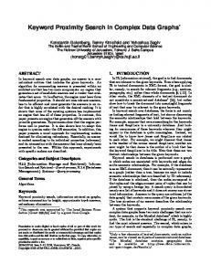
for. In the other conditions both such measures do not decrease rapidly with increasing error and they are quite high throughout. For the sake of brevity, in Tables 1 and 2 only the results retained in 1, 10, 30 runs of the algorithm are displayed: the performance measures show an improvement when the number of runs increases, as expected. From the detailed analysis of all the results (not fully shown here), it comes out that a good performance is reached already when the optimal solution is retained over 10 runs of the algorithm and for 30 runs it generally becomes stable; for greater numbers of runs the performance does not generally increase significantly in terms of recovery of the true partition and goodness of fit. 6. Two Illustrative Applications 6.1 Social Network Data: Monk Data The model proposed has been fitted to sociometric data related to a social network in a monastery (Fershtman 1997) in order to reveal the existence of cohesive groups about social relations. According to Fershtman, S.F. Sampson originally collected the data of a social network among 18 monks in a monastery and found four groups in the network: Young Turks (monks 1, 2, 7, 12, 14, 15, and 16), Loyal Opposition (monks 4, 5, 6, 9, and 11), Outcasts (monks 3, 17, 18), Waverers (monks 8, 10, 13). Reitz (1988) also analyzed the data, constructing a valued network where the choice interaction intensity, representing the strength of the social relationship between individuals, is given in four graded scores: 0.25, 0.5, 0.75, 1. Fershtman (1997) applied an algorithm to such a sociomatrix searching for S-cliques (based on a segregation matrix index) and found three cliques: (A) consisting of a subclique of monks (1, 2, 7, 12) plus three other monks (Young Turks group); (B) corresponding to the Loyal Opposition group plus a Waverer (monk 8); (C) coincident with the Outcasts group. Monks 10 and 13 do not belong to any clique. In order to fit the model proposed here, the asymmetric choice intensities have been converted into dissimilarities by taking the complements to 1 of the original values, so that each dissimilarity measures the weakness of the social interaction between individuals. The symmetric and the skew-symmetric components account for the 96.49% and 3.51% of the total variability, respectively and since the asymmetry of the social relations is structural, it cannot be ignored, as also evident from the pattern of the asymmetry in the heat map of the dissimilarity matrix in Figure 2.

Classification of Asymmetric Proximity Data Table 1. Simulation study: sample size equal to 15

#Random starts

Average MRand

%MRand=1

Average # of iterations

Average loss

Average VAF

Low

1

0.9396

84

2.27

0.2532

0.9157

0.9555

10

0.9686

89

2.22

0.2460

0.9321

0.9647

30

0.9686

89

2.22

0.2460

0.9321

0.9647

1

0.7661

42

2.61

0.3790

0.7650

0.8715

10

0.7682

42

2.67

0.3607

0.7664

0.8722

30

0.7614

42

2.76

0.3596

0.7658

0.8718

1

0.5281

7

3.13

0.4582

0.6154

0.7831

10

0.5695

10

3.07

0.4291

0.6251

0.7891

30

0.5596

10

3.03

0.4263

0.6236

0.7882

1

0.9939

99

2.31

0.0750

0.9603

0.9798

10

1

100

2.30

0.0734

0.9630

0.9813

30

1

100

2.30

0.0734

0.9630

0.9813

1

0.9070

82

2.46

0.1749

0.8691

0.9311

10

0.9836

94

2.50

0.1632

0.8959

0.9462

30

0.9836

94

2.50

0.1632

0.8959

0.9462

1

0.7425

39

3.09

0.2996

0.7276

0.8520

10

0.8118

49

3.10

0.2807

0.7463

0.8630

30

0.8165

49

3.11

0.2806

0.7481

0.8640

1

0.9846

98

2.08

0.0385

0.9631

0.9809

10

1

100

2.08

0.0338

0.9699

0.9848

30

1

100

2.08

0.0338

0.9699

0.9848

1

0.9300

88

2.30

0.0962

0.9040

0.9501

10

0.9979

99

2.26

0.0817

0.9258

0.9622

30

0.9979

99

2.26

0.0817

0.9258

0.9622

Medium 1%

High

Low

Medium 5%

High

Low

Medium 11%

High

Average Cophenetic

Error Level

Average Degree of Asymmetry

Sample size n= 15

1

0.8262

63

2.83

0.1913

0.7921

0.8893

10

0.8936

70

2.79

0.1778

0.8046

0.8965

30

0.8976

70

2.90

0.1775

0.8049

0.8967

D. Vicari Table 2. Simulation study: sample size equal to 35

#Random starts

Average MRand

%MRand=1

Average # of iterations

Average loss

Average VAF

Low

1

0.9944

99

2.14

0.3335

0.9392

0.9689

10

1

100

2.13

0.3311

0.9432

0.9712

30

1

100

2.13

0.3311

0.9432

0.9712

1

0.8996

79

2.56

0.5716

0.7972

0.8895

10

0.9940

95

2.51

0.5504

0.8532

0.9236

30

0.9940

95

2.51

0.5504

0.8532

0.9236

1

0.6607

14

3.51

0.7512

0.4794

0.6889

10

0.7706

22

3.62

0.7352

0.5116

0.7125

30

0.7649

23

3.48

0.7350

0.5104

0.7115

1

0.9567

91

2.32

0.1289

0.9178

0.9562

10

1

100

2.25

0.1037

0.9504

0.9749

30

1

100

2.25

0.1037

0.9504

0.9749

1

0.9143

83

2.40

0.2863

0.8200

0.9028

10

1

100

2.33

0.2487

0.8728

0.9342

30

1

100

2.33

0.2487

0.8728

0.9342

1

0.8136

64

2.95

0.5179

0.5999

0.7721

10

0.9956

95

2.81

0.4784

0.6610

0.8128

30

0.9956

95

2.81

0.4784

0.6610

0.8128

1

0.8992

79

2.36

0.1051

0.8856

0.9381

10

1

100

2.18

0.0486

0.9533

0.9764

30

1

100

2.18

0.0486

0.9533

0.9764

1

0.9226

84

2.46

0.1376

0.8700

0.9306

10

1

100

2.33

0.0973

0.9180

0.9581

30

1

100

2.33

0.0973

0.9180

0.9581

1

0.8497

72

2.75

0.3398

0.6885

0.8278

10

1

100

2.66

0.2907

0.7444

0.8627

30

1

100

2.66

0.2907

0.7444

0.8627

Medium 1%

High

Low

Medium 5%

High

Low

Medium 11%

High

Average Cophenetic

Error Level

Average Degree of Asymmetry

Sample size n= 35


For social network type data that are dominated by clusters, the parsimonious models to fit both the symmetric and the skew-symmetric dissimilarities seem to be better suited than model (3) and (9), respectively; in fact, for this data the non restricted models have been also applied and resulted into the same partition. Firstly, only the symmetrized dissimilarity data have been clustered by fitting a partition with only two levels as in model (5). For any choice of the number of clusters (from 1 to 6) the best partition in 100 runs from different random starting membership matrices has been retained and from the scree plot of the loss function values, the solution corresponding to c=4 has been considered. In Figure 3 two graphical independent representations are overlaid: the dendrogram displays the partition into 4 clusters from the symmetrized data together with the approximation of the skew-symmetric dissimilarities when only one cluster is assumed for the skew-symmetric component (see Remark 2). The lengths of the leaves (vertical dashed lines) represent the average skew-symmetric dissimilarities of the choices of each individual regardless the chosen individuals and do not affect the partition, but only approximate the directed average differential intensities. The vertical dashed branches are just attached to the tree obtained from S to graphically represent the asymmetries similarly to the rationale behind the graphical representations from the slide-vector model (Zielman and Heiser 1993) and drift-vector model (Carroll and Wish 1974). The partition accounts for the 95.88% of the symmetrized dissimilarities, but the average skewsymmetric dissimilarities regardless the clusters account only for the 18.18% of K. From the lengths of the dashed branches we may observe that Monk 2 has been chosen on average with much larger intensity than the converse, regardless the presence of possible groups of monks. The partition in Figure 3 coincides with the three cliques found by Fershtman (1997) plus the singleton formed by Monk 10 that had not been assigned to any group by Fershtman. Furthermore, the parsimonious models (3) and (13) for the symmetric and skew-symmetric component, respectively have been fitted by assuming a common partition and the constrained case only for the between asymmetries (matrix B). The algorithm minimizing the loss function (15) has been run as above: for any choice of the number of clusters (from 1 to 6) the best partition in 100 runs from different random starting membership matrices has been retained and even in this case, by analyzing the scree plot of the loss function values, the partition into c=4 clusters has been selected and displayed in Figure 4. In order to provide empirical evidence about the local minimum problem, the probability to get the partition which attains the minimum

D. Vicari

1 2 3 4 5 6 7 8 9 10 11 12 13 14 15 16 17 18

0.9 0.8 0.7 0.6 0.5 0.4 0.3 0.2 0.1 1 2 3 4 5 6 7 8 9 10 11 12 13 14 15 16 17 18

Figure 2. Monk data: Heat map of the dissimilarity data

0.8 0.6 0.4 0.2 0 -0.2 17 18 3 13 1 16 2 15 7 14 12 10 4 5 6 8 9 11

Figure 3. Monk data: Partition into 4 clusters from symmetric data and lengths proportional to the average skew-symmetric dissimilarities


0.8 0.6 0.4 0.2 0 -0.2 17 18 16 2 15 14 12 7 1 3 13 4 5 8 6 11 10 9

Figure 4. Monk data: Tree of the partition into 4 clusters (Asymmetric data)

observed loss value in a single trial has been estimated in 100 trials ( pˆ  0.51 ) when the algorithm starts from rational partitions as suggested by Vichi (2008), while when it starts from random partitions, such a probability is slightly smaller ( pˆ  0.44 ); thus, in such an application even only 14 or 18 replications, could be enough to get at least one success with probability 1, depending on the starting partitions. The common partition accounts for the 92.48% and the 51.37% of the symmetric and skew-symmetric dissimilarities, respectively, while the partition found by Fershtman accounts only for the 34.44% of the skewsymmetries. When comparing with Figure 3, we note that in the tree of Figure 4 the four clusters are still evident and the heights where they merge are not differently shifted, because the estimated between skew-symmetry is nearly null. This means that the four groups of Monks result quite segregated from each other in terms of intensity of social interactions and represent cohesive groups with internal social relations but rather isolated. Thus, from both Figures 3 and 4 we can see that the Loyal Opposition group is split into two subgroups: Cluster 3 formed by Monks 4, 5 plus a Waverer (Monk 8) and Cluster 4 formed by Monks 6, 9, 11 plus a Waverer (Monk 10). Moreover, the first cluster corresponds to the Young Turks group except for Monk 1 plus two out of the Outcasts.

D. Vicari

As far as the social interactions within groups, the within skewsymmetric component W jointly provides the different lengths of the leaves (vertical dashed lines). Each dashed line below zero (due to a positive value wit) indicates an individual surplus (credit), i.e. the corresponding individual i originates an average “out-dissimilarity” directed within cluster t he belongs to, which is larger than his “indissimilarity” (i.e. within group t Monk i is chosen on average with larger intensity than he chooses); conversely, a dashed line above zero (due to a negative value wit) means a deficit (debit): that monk often chooses individuals within his group more than he is chosen. Since the partition correspond to groups socially isolated, the general asymmetry is due to the within interactions and for example, in the first cluster Monk 2 has been chosen by the other Young Turks with much larger intensity than the converse, while within Cluster 3 Monk 8 shows a “debit” of choices: he has actually chosen with much larger intensity than he has been chosen by the other two Loyal Opposition group members. Monk 11 exhibits a balance of choices, because he chooses with the same average intensities as he is chosen within his group (the length of the corresponding dashed line is zero). Finally, we can consider that the partition fitting jointly the symmetric and skew-symmetric data better manages to detect cohesive groups in the social network, that is groups of individuals, among whom the relationships are relatively frequent, high, intense, strong, or important in comparison with the relationships between members in different groups. 6.2 Confusion Data: Morse Code Signals The well-known confusion data on Morse code signals are investigated. The original data represent the confusion rates among the 36 Morse Code signals (A to Z and 0 to 9) originally collected by Rothkopf (1957). In order to fit the model for clustering asymmetric data, the original data have been converted into dissimilarities by taking the complements to the maximum observed value, so that each dissimilarity measures the rate (x 1000) of correct recognition of a pair of ordered signals. The symmetric component accounts for the 99.67% of the total variability, so in this case the asymmetry degree is not prominent, but it is known for such data that asymmetries are not purely random but reflect a systematic structure. As before, both the symmetrized and the asymmetric dissimilarities have been analyzed: for any choice of the number of clusters (from 1 to 7) the best partition in 100 runs from different random starting membership matrices has been retained for both cases and from the scree plots of the loss function values the corresponding solutions into 5 clusters have been selected (Figures 5 and 6). It is clear from the relative lengths of the leaves


in the trees, which are proportional to the average skew-symmetries, that the asymmetric component of the data is much less relevant than the symmetric one. The symmetrized dissimilarities determine clusters of codes which differ primarily with respect to the number of components (dots and/or dashes) in each signal and the relative preponderance of dots versus dashes among those components. Actually, all the short and simple codes belong to the same cluster, while the longest ones belong to different clusters which reflect the complexity of the signals. Actually, they reflect the MDS configuration in 2 dimensions from the symmetrized dissimilarities and its interpretation widely analyzed by many researchers (see Borg and Groenen 2005 and Saito and Yadohisa 2005). From Figure 5, we note that on average the big contributors to the asymmetry are signals 2 (+21.67), Y (+20.42), P (+20.00) and 5 (-22.22), U (-21.25), H(-16.94) because of their high average asymmetry degrees, but for them we cannot identify the codes which such confusions are directed to. Let us focus on the derived asymmetric clustering structure displayed in Figure 6 which can be better interpreted by considering the information on the number of components (i.e., the number of dots plus the number of dashes) and the ratio of the number of dots to the number of dashes (that is, which type of components is more predominant) in a signal (see Buja and Swayne 2002 for an extensive discussion). In Figure 6 from the top: - Cluster 1 contains 7 codes of medium average length in seconds, formed by many components (4 or 5) with much more dots and fewer dashes; - Cluster 2 consists of 12 short simple signals (with two or three components and average length equal to 0.34 sec including the periods of silence) with generally more dots than dashes; - Cluster 3 includes 7 codes with more components and generally more dashes than dots (except for the simplest and shortest code E) mostly starting with dashes. Such codes present the smallest variability of the within average confusions as evident from the short lengths of the dashed branches; - Cluster 4 contains 6 codes formed by 4 or 5 components having on average the same short and long beeps; - Cluster 5 consists of 4 long codes (the average length is 0.65 sec) formed by 4 o 5 components with more dashes than dots, mostly starting with a dot. Such codes exhibit the largest within average confusion. A greater variety of signals in turn leads to more confusion (cf. Buja and Swayne 2002), as evident from the high level of the within asymmetry present in Clusters 1 and 5 containing the most complex

D. Vicari

-M . E .. I -. N T .A ..- U ... S ...- V .... H .....5 ....-4 ..-. F .-. R --. G .-- W --- O -.- K -.. D .--. P .----1 ..---2 ...--3 -----0 ----.9 .--- J .-.. L --.- Q -..- X -.-- Y --.. Z -.-. C -... B -....6 ---..8 --...7 0

100

200

300

400

500

600

700

800

900

Figure 5. Morse data: Partition into 5 clusters from symmetric data and branch lengths proportional to the average skew-symmetric dissimilarities

.... H -....6 .....5 ....-4 -..- X ...- V -... B -M ..-. F .-- W .-.. L ..- U ... S .-. R .. I -. N -.- K -.. D .A ---..8 T --- O -----0 ----.9 --. G . E .--. P -.-- Y --.. Z --...7 ...--3 -.-. C .--- J --.- Q ..---2 .----1 -100

0

100

200

300

400

500

600

700

800

Figure 6. Morse data: Tree of the partition into 5 clusters (Asymmetric data)

Classification of Asymmetric Proximity Data Table 3. Morse data: Fitted asymmetric dissimilarities between clusters Cluster

1

2

3

4

5

1

0

806.38

847.03

823.95

826.28

2

795.76

0

841.72

818.64

820.97

3

828.97

834.28

0

754.66

756.99

4

852.05

857.36

800.82

0

644.84

5

849.72

855.03

798.48

640.16

0

codes in terms of number of components and lengths. Specifically, the big contributors to the asymmetry within clusters are the codes X (+90.71), 2 (+56.25), 1 (+53.75) and J (-122.50), H (-87.14), Z (-71.67) where, for example, 2 (2: . ._ _ _) have a “credit” which means: low confusions with the other signals in the same cluster when it is the first signal in time, while code J (J: . _ _ _) is more confusable (generates higher confusions) when it is the first signal in time than the reverse. Thus, the sequence (2 J)  (. ._ _ _ . _ _ _ ) causes much lower confusion than (J 2) (. _ _ _ . ._ _ _) as confirmed by the observed data. Note that since matrix W sums to zero by column, the dashed branches in Figure 6 are proportional to the within skew-symmetries, but on average they do not influence the lengths of the between dissimilarities. Cluster 1 (B,H,V,X,4,5,6) exhibits the lowest between skewsymmetry as evident in Figure 6 because its aggregation level is nearly coincident with the corresponding dotted line indicating the average heterogeneity of Cluster 1: on average such codes form an isolated group producing low confusion rates with the other groups, while, the highest levels of the average between skew-symmetries pertain to Clusters 3 and 4. The fitted asymmetric dissimilarities between clusters (Table 3) reveal that the two most similar clusters of codes in terms of average amount of confusions are Clusters 4 and 5 both consisting of codes with many components but different features, with a slight stronger tendency of confusion from long codes having generally the same short and long beeps (for example P, Z) to the longest codes with more dashes than dots (for example J, 2) than the confusion in the opposite direction. Both the short simple signals (Cluster 2) and the codes with generally more dashes than dots (Cluster 3) have a similar average small amounts of confusions, but their different features determine non-confusable groups. Clusters 3 and 4 exhibit the largest average between skew-symmetric dissimilarity (Table 3) with a stronger tendency of confusion from long

D. Vicari

codes with many components having generally the same short and long beeps (for example P, Z in Cluster 4) to codes with generally many dashes (Cluster 3) than the confusion in the opposite direction. The complexity of the data is better captured when the partition is found by taking into account jointly the rows and the columns of the data. Such clusters identify codes similar on average for amount of confusions and having common directions of confusions on average with codes in the other clusters. Moreover, symmetry and skew-symmetry are cluster-related as emerges from the tree: the largest the average amount of the cluster confusion is, the largest the variability of the within degree of asymmetry is. 7. Conclusions A model has been proposed to cluster asymmetric dissimilarity data when the asymmetry can be assumed to be structural and not due to noise. Such information may strongly affect the clustering process and mask the real degree of the asymmetry of the data, leading to an incomplete and inaccurate analysis if ignored. The model proposed relies on the decomposition of the data matrix into a symmetric and a skew-symmetric component both decomposed into within and between cluster effects. Regardless the types of classification structures assumed for both the symmetric and the skew-symmetric components of the data, the crucial point is that the search for clusters needs to involve both of them, to take into account the amounts and the directions of the data. In such a respect, the model is formalized in a general framework and gives actually rise to a class of models that differ whether or not some effect is included. It is not necessary to model the symmetric part by a clustering model: a form of MDS could also be useful, or alternatively, the average skew-symmetry may be modelled (for example by a drift-vector model) and represented jointly with a standard classification structure for symmetric data. Particular attention has been given to the restricted model where only one partition of the objects is jointly fitted to the symmetric and skew-symmetric components of the data and the applications show that it manages to detect cohesive and interpretable groups of objects with a limited loss of the fit if compared with the separate analyses. The objects in the same cluster share the same amount of exchanges on average (close or similar objects) and the same average imbalance (in terms of intensity and direction) directed to the other clusters. Note that the symmetric part of the data is generally prominent in real applications and since the imbalances are bounded because of the non-negativity of the asymmetries, strong imbalances generally correspond to large amounts between objects. Moreover, the decomposition of the asymmetries into between and within effects results in clusters having similar exchanges between objects within the same cluster, given the average amounts (for example,


exchanges between leader market brands or countries, or between social actors with large relations), while exchanges between clusters refer to objects with generally different average symmetries. Positive (negative) parameters in the estimated matrices B and W allow to identify clusters and objects within each clusters, respectively which are mainly origins (destinations) of the asymmetric exchanges. The model and the algorithm can be easily modified according to possible alternative choices of the clustering structures to fit the symmetric component of the data, by imposing different order constraints on the matrices identifying the classification structures. Alternative options like genetic algorithms, simulated annealing and other meta heuristics could be also employed as alternatives to the multistart strategy to handle the problem of local minima. References ARABIE, P., SCHLEUTERMANN, S., DAWS, J., and HUBERT, L. (1988), “Marketing Applications of Sequencing and Partitioning of Nonsymmetric and/or Two-Mode Matrices”, in Data Analysis, Decision Support and Expert Knowledge Representation in Marketing, eds. W. Gaul and M. Schader, Hiedelberg: Springer Verlag, pp. 215–224. BORG, I., and GROENEN, P. (2005), Modern Multidimensional Scaling. Theory and Applications (2nd ed.), Berlin: Springer. BOTH, M., and GAUL, W. (1986), “Ein Vergleich Zweimodaler Clusteranalyseverfahren”, Mathematical Methods of Operations Research, 57, 593–605. BROSSIER, G. (1982), “Classification Hiérarchique à Partir de Matrices Carrées Non Symétriques”, Statistiques et Analyse des Données, 7, 22–40. BUJA, A., and SWAYNE, D.F. (2002), “Visualization Methodology for Multidimensional Scaling”, Journal of Classification, 19, 7–44. CARROLL, J.D., and WISH, M. (1974), “Multidimensional Perceptual Models and Measurement Methods”, in Handbook of Perception (Vol. II), eds. E.C. Carterette and M.P. Friedman, New York: Academic, pp. 391–447. CONSTANTINE, A.G., and GOWER, J.C. (1978), “Graphic Representations of Asymmetric Matrices”, Applied Statistics, 27, 297–304. DESARBO, W.S. (1982), “GENNCLUS: New Model for General Non-Hierarchical Clustering Analysis”, Psychometrika, 47, 449–475. DESARBO, W.S., and DE SOETE, G. (1984), “On the Use of Hierarchical Clustering for the Analysis of Nonsymmetric Proximities”, Journal of Consumer Research, 11, 601– 610. DESARBO, W.S., MANRAI, A.K., and BURKE, R.R. (1990), “A Nonspatial Methodology for the Analysis of Two-Way Proximity Data Incorporating the Distance– Density Hypothesis”, Psychometrika, 55, 229–253. DE SOETE, G., DESARBO, W.S., FURNAS, G.W., and CARROLL, J.D. (1984), “The Estimation of Ultrametric and Path Length Trees from Rectangular Proximity Data”, Psychometrika, 49, 289–310. ECKES, T., and ORLIK, P. (1993), “An Error Variance Approach to Two-Mode Hierarchical Clustering”, Journal of Classification, 10, 51–74. ESCOUFIER, Y., and GRORUD, A. (1980), “Analyse Factorielle des Matrices Carrées Non-Symetriques”, in Data Analysis and Informatics, eds. E. Diday et al., North Holland: Amsterdam, pp. 263–276.

D. Vicari FERSHTMAN, M. (1997), “Cohesive Group Detection in a Social Network by the Segregation Matrix Index”, Social Networks, 19, 193–207. FURNAS, G.W. (1980), “Objects and Their Features: The Metric Representation of Two Class Data”, unpublished doctoral dissertation, Stanford University. FUJIWARA, H. (1980), “Methods for Cluster Analysis Using Asymmetric Measures and Homogeneity Coefficient”, The Japanese Journal of Behaviormetrics, 7, 12–21. GOWER, J.C. (1977), “The Analysis of Asymmetry and Orthogonality”, in Recent Developments in Statistics, eds. J.R. Barra, F. Brodeau, G. Romier, and B. Van Cutsem, North Holland: Amsterdam, pp. 109–123. HUBERT, L. (1973), “Min and Max Hierarchical Clustering Using Asymmetric Similarity Measures”, Psychometrika, 38, 63–72. HUBERT, L., and ARABIE, P. (1985), “Comparing Partitions”, Journal of Classification, 2, 193–218. HUBERT L.J., ARABIE P., and MEULMAN J. (2001), Combinatorial Data Analysis: Optimization by Dynamic Programming, Philadelphia: SIAM. HUBERT L.J., ARABIE P., and MEULMAN J. (2006), The Structural Representation of Proximity Matrices with MATLAB, Philadelphia: SIAM. MCCORMICK, W.T., SCHWEITZER, P.J., and WHITE, T.W. (1972), “Problem Decomposition and Data Reorganization by a Clustering Technique”, Operations Research, 20, 993–1009. OKADA, A. and IWAMOTO, T. (1996), “University Enrollment Flow Among the Japanese Prefectures: A Comparison Before and After the Joint First Stage Achievement Test by Asymmetric Cluster Analysis”, Behaviormetrika, 23, 169–185. OZAWA, K. (1983), “Classic: A Hierarchical Clustering Algorithm Based on Asymmetric Similarities”, Pattern Recognition, 16, 201–211. REITZ, K.P. (1988), “Social Groups in a Monastery”, Social Networks, 10, 343–357. ROCCI, R. and BOVE, G. (2002), “Rotation Techniques in Asymmetric Multidimensional Scaling”, Journal of Computational and Graphical Statistics, 11, 405–419. ROTHKOPF, E.Z. (1957), “A Measure of Stimulus Similarity and Errors in Some Paired Associate Learning”, Journal of Experimental Psychology, 53, 94–101. RUBIN, J. (1967), “Optimal Classification into Groups: An Approach to Solve the Taxonomy Problem”, Journal of Theoretical Biology, 15, 103–144. SAITO, T., and YADOHISA, H. (2005), Data Analysis of Asymmetric Structures. Advanced Approaches in Computational Statistics, New York: Marcel Dekker. SOKAL, R.R., and ROHLF, F.J. (1962), “The Comparison of Dendrograms by Objective Methods”, Taxon, 11, 33-40. SHEPARD, R.N., and ARABIE, P. (1979), “Additive Clustering: Representation of Similarities as Combinations of Discrete Overlapping Properties”, Psychological Review, 86, 87–123. TAKEUCHI, A., SAITO, T., and YADOHISA, H. (2007), “Asymmetric Agglomerative Hierarchical Clustering Algorithms and Their Evaluations”, Journal of Classification, 24, 123–143. VICARI, D., and VICHI M. (2000), “Non-Hierarchical Classification Structures”, in Data Analysis, Studies in Classification Data Analysis and Knowledge Organization, eds. W. Gaul, O. Opitz, and M. Schader, Berline: Springer, pp.51–66. VICHI, M. (2008), “Fitting Semiparametric Clustering Models to Dissimilarity Data”, Advances in Data Analysis and Classification, 2, 121–161. YADOHISA, H. (2002), “Formulation of Asymmetric Agglomerative Hierarchical Clustering and Graphical Representation of Its Result”, Bulletin of the Computational, Statistics of Japan, 15, 309–316. ZIELMAN, B., and HEISER, W.J. (1993), “Analysis of Asymmetry by a Slide-Vector”, Psychometrika, 58, 101–114.

Classification of Asymmetric Proximity Data ZIELMAN, B. and HEISER, W.J. (1996), “Models for Asymmetric Proximities”, British Journal of Mathematical and Statistical Psychology, 49, 127–146.