Classification of Heterogeneous Gene Expression Data - sigkdd

Classification of Heterogeneous Gene Expression Data Benny Y. M. Fung

Vincent T. Y. Ng

Department of Computing,

Department of Computing,

The Hong Kong Polytechnic University,

The Hong Kong Polytechnic University,

Hung Hom, Kowloon, Hong Kong

Hung Hom, Kowloon, Hong Kong

[email protected]

[email protected]

ABSTRACT Recent advanced technologies in DNA microarray analysis are intensively applied in disease classification, especially for cancer classification. Most recent proposed gene expression classifiers can successfully classify testing samples obtained from the same microarray experiment as training samples with the assumption that the symmetric errors are constant among training and testing samples. However, the classification performance is degraded with heterogeneous testing samples obtained from different microarray experiments. In this paper, we propose the “impact factors” (IFs) to measure the variations between individual classes in training samples and heterogeneous testing samples, and integrate the IFs to classifiers for classification of heterogeneous samples. Two publicly available lung adenocarcinomas gene expression data sets are used in our experiments to demonstrate the effectiveness of the IFs. It shows that, with the integration of the IFs to the Golub and Slonim (GS) and k-nearest neighbors (kNN) classifiers, the classifiers can be further improved on the classification accuracy of heterogeneous samples. Even more, the classification accuracy of the integrated GS classifier is around 90%.

Keywords Gene expression data, classification, significance analysis of microarrays

feature

selection,

1. INTRODUCTION Recent advanced technologies in DNA microarray analysis allow us to examine gene expression levels for a huge amount of genes in a single experiment. Different data mining techniques are used to analyze and discover knowledge from gene expression data. Since the number of examined genes in an experiment is in term of thousands, data mining techniques have been intensively applied in the analysis of gene expression data [6]. Microarray data contain two kinds of errors, namely symmetric and random errors [12], and normalization is a common technique to minimize the symmetric errors. Symmetric errors are defined as controllable errors which induce almost-equally variations at microarray experiments [5], and random errors are defined as uncontrollable errors which induce different degrees of variations at microarray experiments by chance. Normalization is a common pre-processing step to remove or minimize the influence of the symmetric errors and achieve data centralization. Some common approaches are global normalization, log-transformation, regression normalization, intensity-dependent normalization, and etc. Data centralization is a symmetry property of any two samples whose genes have equal or similar ratio of their expression levels. The objective is to identify a symmetry line

SIGKDD Explorations.

among the gene expression levels of two samples, and transforms asymmetric gene expression levels into symmetric one with a transformation function [18]. Unfortunately, there is no efficient way to eliminate the random errors [15]. The symmetric errors are constant among samples in the same microarray experiments, but samples in different experiments have different symmetric errors. The symmetric errors within a microarray experiment can be considered as intra-experimental variations. Suppose that there are different data sets obtained by different microarray experiments, and then the symmetric errors of these data sets are different [21]. Hence, the differences of experimental variations among different microarray experiments can be defined as inter-experimental variations. When we consider a combined data set of data sets from different microarray experiments, most normalization approaches, which work fine for a single data set, are incompatible for normalizing such combined data set because there are inter-experimental variations. Assume that the annotation of accession numbers and number of genes are the same. Practically, we can merge the data sets by appending, but this merging does not consider the interexperimental variations, and thus the variations are distributed and shared over other data sets. The final result is like the one after an averaging process. That is, data sets originally with fewer variations are become unstable since data sets with more variations distribute their variations to them. In this paper, we propose the “impact factors” (IFs) to measure the variations between individual classes in training samples and heterogeneous testing samples obtained from different microarray experiments, and then integrate the IFs to classifiers for classification of heterogeneous samples. The reminder of this paper is organized as follows. We review classification approaches of gene expression data in section 2. Among different classifiers, we discuss the Golub and Slonim (GS) classifier in section 3 since it is one of the recent proposed classifiers, designed for classification of gene expression data with biological relevance [16]. Furthermore, we adopt the significant analysis of microarrays (SAM) (i.e. a feature selection method) to select features at IFs computation [19], and the details are described in section 4. In section 5, we present the algorithm of the IFs. Experimental results are presented and discussed in section 6. Finally, we give our concluding remarks and future works.

2. RELATED WORKS Several publications have done a comprehensive review on the progress of cancer classification [6], [11]. Their works involve of reviewing a number of traditional and microarray-specified feature selection methods and classification approaches. For the classification with machine learning approaches, support-vector

Volume 5,Issue 2 - Page 69

machines (SVM) [1], artificial neural network (ANN) [22], knearest neighbors (kNN) [11], and self-organizing map (SOM) [9] have been successfully applied to cancer classification. Their classification performances with different distance metrics, like Pearson correlation, Euclidean distance, cosine coefficient and signal-to-noise distance, are compared [6]. In addition, other approaches are Fisher linear discriminant analysis (FLDA) [9], CAST [3] and boosting [2]. Since gene expression data have a huge amount of genes, feature selection and extraction methods are used to find informative genes. These methods include principal component analysis, linear discriminant analysis, projection pursuit, and etc. A comprehensive review of feature selection and extraction methods can be found in Jain et al. [10].

3. GOLUB AND SLONIM (GS) CLASSIFIER A binary-class classifier, especially designed for classification of binary gene expression data, is called Golub and Slonim (GS) classifier [16]. Among different classifiers, only tree-based (i.e. boosting) and partitioning-based (i.e. GS classifier) classifiers have the interpretation of biological relevance by the means of revealing the relationships between genes in a step-wise approach [11]. The processes of splitting a whole data set into a number of smaller subsets and performing correlation analysis on these smaller subsets provide insight understanding of selection mechanism and correlation analysis among genes. Other nonbiological relevance classifiers, like ANN, SVM, and CAST, consider whole gene expression data as a set of distribution and perform classification based on the distribution of gene expression levels without the consideration of individual relationships among genes, and their correlation analysis is encapsulated in a “black box”, implying that it is difficult to analyze biological relevance. Here, we describe the approach of the GS classifier. The first step is to calculate the “signal-to-noise” (SNR) distance for genes. Assume that the expression levels of gene g in n training samples be represented by an expression vector g=(e1, e2, …, en), where ei donates the expression level of g in tuple i, c={Normal, Cancer} be the class vector donating the classes of tuple i, and (µNormal(g), σNormal(g)) and (µCancer(g), σ Cancer(g)) be the class mean expression level and standard deviation of g in normal and cancer classes. First of all, g is normalized across samples with the mean expression level µ(g) and standard deviation σ(g) of the gene. The SNR of g is:

µ Normal ( g ) − µ Cancer ( g ) (1) σ Normal ( g ) − σ Cancer ( g ) The second step is to construct two class-vectors to represent the overall similarities of testing sample Y to normal and cancer classes, respectively. From the SNR-values, a positive SNR-value represents that the gene is in normal class, while a negative SNRvalue represents that the gene is in cancer class [16]. Very often, certain representative genes are sufficient to represent the overall similarities of the classes. Hence, only k/2 genes having the highest and lowest SNR-values are selected and expressed as sets Gk-highest and Gk-lowest to represent the overall similarities for the corresponding classes, when k genes are required. Assume that avg(g) be the average value of the class mean expression levels of normal and cancer classes for gene g (i.e. avg(g)=(µNormal(g)+ µCancer(g))/2). A similarity measure called vote factor, v(g), is calculated for g in Y by v(g)=SNR(g)*[Yg-avg(g)], where Yg is the SNR ( g ) =


normalized gene expression levels of g in Y with respects to the

µ(g) and σ(g) of the same gene in the training samples. The overall similarities corresponding to the classes, which are expressed as Vpositive and Vnegative for normal and cancer classes, are the sum of k/2 positive and negative v-values (i.e. Vpositive=Σ(v(g)|(v(g)>0)∧(g∈Gk-highest)) and Vnegative=Σ(v(g)|(v(g)< 0)∧(g∈Gk-lowest))). The testing sample is classified as normal for |Vpositive|>|Vnegative|. If otherwise, it is classified as cancer. Since Vpositive and Vnegative are in absolute distance, the relative difference, which is called prediction strength (PS), between them is calculated (in equation 2). If the PS is sufficiently large, the assigned class label is confirmed. Otherwise, the new sample is classified as “uncertain”. PS =

max(V positive , Vnegative ) − min(V positive , Vnegative ) V positive + V negative

4. SIGNIFICANCE ANALYSIS MICROARRAYS (SAM)

(2)

OF

A feature selection method called Significance Analysis of Microarrays (SAM) has been proposed by Tusher et al. to identify significant genes in microarray experiments based on the variations of the standard deviations in repeated measurements [19]. It aims at measuring fluctuations of the expression levels for a gene across a number of microarray experiments. It first calculates an observed relative difference, dr(g), for gene g in training samples X based on the ratio of change in gene expression to standard deviation for that gene. When using the same terminology as the GS classifier, dr(g) is: dr (g) =

µ Normal ( g ) − µ Cancer ( g )

(3)

s( g ) + s 0

where s(g) is a measurement of variations for gene g (in equation 4), and s0 is a factor to adjust the s(g) because of small sample size [7]. β is the average number of measurements in both classes.

s( g ) = β × {∑[ X g − µ Normal ( g )]2 + [ X g − µCancer ( g )]2 } 1

, where β =

Normal

+ 1

Cancer

Normal + Cancer − 2

(4)

SAM uses a technique of permutations of the repeated measurements to identify significant genes. The idea is to assume that a significant gene in a class should have differential expression levels over another class. However, after a certain number of permutations, such differentiations between two (1) classes are eliminated because the permutations re-arrange the gene expression levels of both classes. After p permutations, it calculates a permuted relative difference, dp(g), for gene g. As a result, there are p dp(g)’s for the gene, and the mean relative difference, dE(g), for gene g over p permutations is calculated [19]. d E (g) =

∑d

p (g)

(5)

p

dE(g) is used as a reference point to identify those genes with differential expression levels, which are called significant genes in this context. For a significant gene, its dE(g) should be comparably different from its dr(g). A threshold, which is the distance in both directions away from a straight line with slope


When the threshold value is set, the smallest positive dr(g) and least negative dr(g) are used as cutoff lines to predict the number of falsely-significant genes for the corresponding threshold value. The number of predicted falsely-significant genes for dr(g) is computed by counting the number of genes at its dp(g)’s that exceed the cutoff lines. Finally, the number of predicted falselysignificant genes for the threshold value is the average number of predicted falsely-significant genes for all dr(g)’s.

5. IMPACT FACTORS We propose the impact factors (IFs) to measure the variations between individual classes in training samples and a heterogeneous testing sample obtained from different microarray experiment. The rationale is to measure the inter-experimental variations (i.e. the differences between two microarray experiments) based on the significant genes in the training samples, and set up individual reference points corresponding to classes in the training samples from the extracted significant genes. Every reference point is then used to calculate its own relative scaling factor for the corresponding class, and this factor is used to rescale the gene expression levels in the testing sample with respects to the reference point of that class individually. With the rescaled expression levels, relative distances to the training samples are calculated. In order to enhance the discriminative powers of the IFs, only those genes with a higher relative difference are selected and integrated to classifiers for classification of heterogeneous sample. Figure 1 shows the algorithm of IFs computation.

values against the number of predicted falsely-significant genes, and the optimal threshold value is chosen at the convergence point. 16 Falsely-significant genes

equal to 1 across the origin, is used to exclude the insignificant genes, which are enclosed by the range.

14 12

The initial point of convergence: the number of falsely-significant genes is smallest.

10 8 6 4 2 0 1

1.2

1.4

1.6

1.8

Threshold Delta value

Figure 2. Selection of the optimal threshold value. With the feature selection method, significant genes are extracted from original genes in training samples. Assume that sets G and G’ be the sets of original and extracted significant genes, and hence we have G’⊂G. For each g∈G’, we calculate class trimmean expression level. In a k% trim-mean value, data members are sorted, and k/2% data members at each end of the sorted list are discarded. The k% trim-mean value is then calculated from those un-discarded members only. The idea of the trim-mean value is to eliminate outliners. We choose 30% of data members to be trimmed, the 30% class trim-mean expression levels are expressed as µ’Normal(g) and µ’Cancer(g) for each extracted significant gene g, where g∈G’, in normal and cancer classes. For heterogeneous samples, handling of missing values and feature alignment are required. Assume that set Gh be the set of genes in a heterogeneous testing sample Yh. In fact, some extracted significant genes may not be existed in Gh (i.e. Gh∩G’⊄G’). The objective is to construct a gene set Gh’ for Yh, and thus Gh’ has the same set of genes as the extracted significant genes G’. (i.e. Gh’⊆G’∩G’⊆Gh’). The feature alignment is performed by looking for some commonly existed genes between Gh and G’ (i.e. Gh’⊆Gh∩G’), while the handling of missing value is done by the nearest neighbor (NN) approach. The training sample with the smallest Euclidean distance to the testing sample is the nearest neighbor, and the gene expression levels in the nearest neighbor are copied to the missing expression levels of the corresponding genes in the testing sample (i.e. Gh’⊆G’/Gh).

Figure 1. The algorithm of IFs computation. In SAM, the number of predicted falsely-significant genes depends on the choice of the threshold values. In our studies, there is a convergence point for the number of predicted falselysignificant genes with an increasing threshold value. At this point, the number of predicted falsely-significant genes becomes minimal, and thus the extracted significant genes at this point have the lowest probability to be falsely-significant. Hence, the optimal threshold value, producing the optimal number of significant genes, corresponding to the smallest number of predicted falsely-significant genes at the convergence point is chosen. For example, Figure 2 shows a graph of the threshold


We estimate relative scaling factors for individual classes in the training samples based on the extracted significant gene set G’ and the constructed gene set for the heterogeneous sample Gh’, acting as reference points to rescale the gene expression levels in the heterogeneous sample. We first calculate baselines of, respectively, normal and cancer classes in the training samples. The baselines for the classes are the sum of all the corresponding class trim-mean expression levels of the significant genes g, expressing as ∑µ’Normal(g) and ∑µ’Cancer(g), where g∈G’, for normal and cancer classes, respectively. Similarly, the baseline for a heterogeneous sample Yh is the sum of gene expression levels of the constructed genes g, expressing as ∑Yhg, where g∈Gh’. Since the relative scaling factors are used to minimize the inter-experimental variations, one possible way to perform the minimization is to amplify or reduce (i.e. rescale) the gene


expression levels of the heterogeneous sample with respects to the reference points of the corresponding individual classes. Thus, the relative scaling factors are ratio of the baselines corresponding to the classes in the training samples to the baseline of the heterogeneous testing sample. They are: RNormal = RCancer =

∑ µ'

g∈G '

∑ µ'

g∈G '

∑Y

(g)

Normal

h

g

(6)

h

g∈G '

Cancer

∑Y

(g)

h

g

(7)

g∈G h '

The relative scaling factors are then used to rescale the gene expression levels in the heterogeneous sample. The magnitudes of RNormal and RCancer define different rescaling operations. When Rc>0, where c∈{Normal, Cancer}, the total expression levels of extracted significant genes of class c in training samples are higher than the total gene expression levels, corresponding to extracted significant genes, in testing sample. Hence, a process of signal enhancement is required. Similarly, signal reduction is required for the case Rc t )}

n d Cancer {g | (r ( g ) > t )} n

(11)

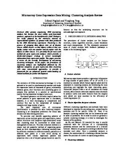
Consider the example of IFs computation in Figure 3. The expression levels of training samples and a heterogeneous sample are listed. First of all, SAM is performed, and significant gene set G’ is extracted. For the heterogeneous sample, significant genes 1071_at and 1319_at are aligned corresponding to the extracted significant genes, and their expression levels are copied to Gh’. Also, significant gene 1439_s_at is missed, and thus NN approach is performed. During the operation, assume that the first sample in cancer class is the nearest neighbor. Therefore, the gene expression level in the nearest neighbor corresponding to the missing gene expression level in the testing sample is copied to Gh’. Even more, RNormal, RNormal, δNormal, and δCancer are calculated in equation 6, 7, 8, and 9. With these fours parameters, the rescaling is performed, and the corresponding dNormal(g) and dCancer(g) are calculated for gene g. Suppose that the threshold value is set to 2 in equation 11 and 12. When calculating the r(g) for gene g, where g∈Gh, only gene 32195_at is included in the IFs computation since other r(g)’s are excluded by the required threshold value.

100_g_at 1071_at 1319_at 1439_s_at 1440_s_at 37659_at 32118_at 32195_at 37033_s_at

Heterogeneous Training samples (G) sample (Gh) Normal Cancer 362 178 296 273 192 272 689 532 250 15 97 194 16 1233 809 546 482 551 221 63 1533 1461 586 240 499 159 35 54 30 10 51 2 362 832 178 272 576 136 -21 200 3424 6519 1170 2042 309 1823 Gh ’ Accession Level 1071_at 16 1319_at 63 1439_s_at 240

G’ Accession µ’Normal(g) µ’Cancer(g) 1071_at 490 102 1319_at 863 418 1439_s_at 1193 299 RNormal 7.98 Gh Accession 1071_at 1319_at 32118_at 32195_at

RCancer 2.57

Level 16 63 -21 100

δNormal

δCancer

1353

520

dNormal(g)

dCancer(g)

r(g)

0.91 0.63 1.12 0.41

0.92 0.69 1.10 0.51

0.01 0.10 0.02 0.24

(12)

where n is the number of the significant genes whose r(g)’s are higher than a required threshold value t. Since dNormal(g) and dCancer(g) are both in absolute values, IFNormal and IFCancer must be non-negative values. The lower-bounds of


5.1 Example

Accession

δ Normal

δ Normal =

IFs are equal to 0. However, the upper-bound of IFs depends on the factor Yhg×Rc, where c∈{Normal, Cancer}. Since this factor is unbounded, the upper-bound is unbounded too.

IFNormal 0.48

IFCancer 0.51

Figure 3. Example of IFs computation.


5.2 Gene Selection Gene selection is a useful preprocessing to select informative genes for classification and hence improves classification performances. In gene expression data, samples have too many genes (i.e. features) associated with them, and many of genes are noisy or irrelevant for the differentiability between normal and cancer classes. Their inclusion in classification not only introduces confusions with informative genes, but also increases computational complexity. The calculation of the IFs only selects a set of informative genes in training samples. The general criterion for the selection is that the genes should have sufficient differentiability between two classes. From previous works, gene selection is mainly achieved by statistical measurements, which can be divided into either correlation or distance measurements. Some common correlation measurements include the Pearson correlation [2] and Spearman correlation [6], while some common distance measurements are the Euclidean distance [11], Cosine coefficient [6], signal-to-noise ratio [9] and ratio of betweengroups to within-groups [8]. Most statistical-based gene selection measurements identify informative genes based on differential expression levels of a gene between two classes, assuming that all genes (i.e. features) are direct-relevant to tissues (i.e. either normal or cancer) of samples. In fact, genes, differentially expressed between two classes, do not always imply that the genes are direct-relevant to tissue of either class since some differential expressions may be caused by different compositions of cell types. In fact, normal and cancer cells have different compositions of cell types (i.e. a kind of biological mechanism), and some genes are also responsible for the mechanisms in the compositions. Some informative genes extracted by the statistical measurements may be caused by the effects of different compositions, instead of direct-relevant to the tissues of either class. This issue is called gene or sample contamination [2], [11]. SAM uses a technique of permutations to minimize biological mechanisms in gene expression data, and extracts informative genes without the inclusion of biological mechanisms. Its significance has been demonstrated by the problem: the transcriptional response of lymphoblastoid cells to ionizing radiation [19].

5.3 Integration of the IFs to Classifiers The impact factors (IFs) are integrated to classifiers so that the integrated classifiers have the capability of classifying heterogeneous samples. The IFs are dissimilarity measures, namely IFNormal and IFCancer, for normal and cancer classes, and they express the inter-experimental variations between the corresponding classes in training samples and heterogeneous testing sample. Bias factors, εNormal and εCancer, are introduced in the integration of the IFs to minimize the impacts of unequal proportions of extracted significant genes among classes. When the expression data are acquired from microarray experiments, it is possible that the proportions of tissue-specific genes, related to normal and cancer classes, are uneven, and hence the proportions of extracted significant genes, identified by SAM, are uneven too. Therefore, the IFs have different degrees of bias according to the classes. As a result, we introduce bias factors in the integration to adjust the importance of the IFs for the corresponding classes. In fact, the possible range of the bias factors is subjective, and may be varied from data sets to data sets.


For most classifiers using similarity/ dissimilarity measures for making classification decisions, one way to perform the integration is to multiply IFs directly to the measures since the IFs are dissimilarity measures. There are two cases for the integration. If there is a dissimilarity measure, the IF of a class is multiplied to the measure with the same class as the corresponding IF. In contrast, if there is a similarity measure, the IF of a class is multiplied to the measure with another class as the corresponding IF. Assume that ddissimilarity and dsimilarity are, respectively, the dissimilarity and similarity measures before the integration, while d’dissimilarity and d’similarity are, respectively, the dissimilarity and similarity measures after the integration. The general approaches of the integration are: d’dissimilarity={ d’similarity={

ddissimilarity×IFNormal×εNormal for normal class (13) ddissimilarity×IFCancer×εCancer for cancer class dsimilarity×IFCancer×εCancer for normal class dsimilarity×IFNormal×εNormal for cancer class

(14)

5.3.1 Golub and Slonim (GS) classifier For the choice of classifiers, we adopt the Golub and Slonim (GS) classifier for the first integration because (1) the GS classifier is specially designed for binary-class gene expression data, and there are two classes of samples in our data sets. It makes the classifier performs well for the classification. (2) The GS classifier calculates features with the “signal-to-noise” distance, which measures variations of a gene between two classes. Also, the SAM measures the variations of a gene between two classes. Hence, the feature selection strategy of the classifier and IFs is similar. (3) The semi-final deliveries of the GS classifier are two vote factors (i.e. Vpositive and Vnegative). Also, there are two dissimilarity measures for the IFs (i.e. IFNormal and IFCancer). The integration is performed by multiplying the IF of a class to the V-value of another class since V-values are similarity measures. Supposed that Vˆpositive and Vˆnegative are the new vote factors to normal and cancer classes, respectively. We have: Vˆ positive = V positive × IFCancer × ε Cancer

(15)

Vˆnegative = Vnegative × IFNormal × ε Normal .

(16)

After the inter-experimental variations are included, the remaining steps are the same as the ordinary GS classifier. The testing sample is classified as normal for | Vˆ positive |>| Vˆnegative | . Similarly, it is classified as cancer for | Vˆ positive |