Hans J. Andersen and Moritz Störring. Computer Vision and Media Technology Laboratory. Institute of Health Science and Technology, Aalborg University.
Classifying Body and Surface Reflections using Expectation-Maximization Hans J. Andersen and Moritz St¨orring Computer Vision and Media Technology Laboratory Institute of Health Science and Technology, Aalborg University Niels Jernes Vej 14, DK-9220 Aalborg, Denmark Email: {hja,mst}@cvmt.auc.dk Abstract This paper presents a new method for the classification of dielectrical object’s RGB values into their body and surface reflections. Instead of segmenting into the two reflection components a weight is estimated that a given pixel belongs to one of them. A weighting value may be useful for classification of body and surface reflections in combination with other methods. The method operates globally on the pixel points using expectation maximization for fitting the body and surface vectors in the case of one highlight reflection. In the case of multiple highlights it is shown that it is possible to relax the method by fitting one surface vector to multiple highlights. The method was empirically validated on real image data captured using a high dynamic imaging sensor (120dB). Promising results show that the method is capable of classifying the two reflection components.
Introduction The aim of many applications is to capture relevant information of an object by analysis of either its body or surface reflections, e.g. analysis of vegetation or skin. The two reflection components are very different in nature and hence for proper analysis of an object’s characteristic it is necessary to classify their content. Body reflection is formed by light penetrating into the material body where it scatters around hitting pigments, fibers and other materials. It is the reflection that gives pertinent spectral information about the object, as the color. Surface reflection is due to the effect that the refractive index between the object and the surrounding is different. Therefor some of the incident light will be reflected directly at the surface before penetrating into the object. Several methods operating locally in the image plane have been proposed for classification of objects’ reflection components [5, 7]. However, in many situations it will not be possible to rely on the spatial context due to the structure of the object, in these cases it will be necessary to classify the reflection components globally in the RGBcube. Globally operating methods have been proposed [5, 8,
12], but these are still limited to one single highlight, i.e. only one surface vector emerging from the body vector. However, objects in every day scenarios may have multiple highlights either due to several light sources or due to their shape. These objects may have multiple surface vectors emerging at different intensity levels of the body vector. Another constrain for physics-based image analysis has been the limited dynamic range of the available cameras. This study demonstrates how a newly introduced 120dB imaging sensor may enable new possibilities within the analysis of reflection components. In this paper we will introduce a method using EM (Expectation-Maximization) for classification of objects reflection components operating globally on their RGB values. The results show that by using EM to fit a body and surface vector it possible to assess the content of reflection for the two component. The method may be used for weighting of other analysis methods that rely on either of the reflection components or for isolation or specific areas on the object of interest for further analysis, i.e. the body reflection may used to obtain pertinent information about an object, the surface reflection for white balancing or control of the image formation process, e.g. exposure time. The paper is organized as follows: The first section presents the dichromatic reflection model together with the EM algorithm. The next focuses one the implemented method. The following sections present the experimental setup, results, discussion, and conclusion.
Modelling The Dichromatic Reflection Model The dichromatic reflection model, introduced by Shafer (1985) [10], states that the reflected light from dielectrical objects may be split into two (di) distinct reflection components from the body (b) and the surface (s) of it. For a color camera the model may be expressed by:
C(x, y) = mb (Θ)Cb (x, y) + ms (Θ)Cs (x, y)
(1)
where C(x, y) is a three dimensional color vector for the pixel at location (x, y). It is an additive mixture of the body reflection Cb (x, y) and the surface reflection Cs (x, y) color vectors of the body and surface reflections scaled by the geometrical scaling factors mb (Θ) and ms (Θ), respectively. Θ, denotes the photo metrical angles, incident angle, exit angle of the illumination, and the phase angle between the camera and observer. For eq. 1 it may also been noted that the pixel points of an object will be distribution in a plane spanned by its body and surface vectors. Further, the chromaticity of the pixel points will traverse from the chromaticity of the body reflection to the chromaticity of the surface reflection at increasing intensity [1]. For analysis of color images the model has been used for image segmentation [5, 9, 7], analysis of highlights [6], estimating scene properties [8], color and characteristic of illumination [1, 15, 11], and for computer graphics rendering [14]. Expectation-Maximization The Expectation-Maximization algorithm (EM) [3] is used for many statistical estimation problems and especially for parameter estimation in incomplete data sets. The basic structure of the method is as follows: • Initialize the parameters, that need to be estimated, randomly or by some intuitively classification of the data set • Iterate until the parameters converge: – E step: Compute the expectation – M step: Update the parameters In this case the objective is to classify the pixels body and surface reflection components, which in nature is an incomplete data sets as we do not have the class assignments given a priori.
Method One highlight In the case of one highlight cluster we expect the pixel points to be distributed in one body and surface reflection cluster, respectively. We approximate these clusters by two vectors, the object’s body and surface reflection vector, respectively. Initialization The EM procedure is initialized by classification of the pixel points into their body (b) and surface (s) reflection components according to their intensity by the following criteria:
( ω(x, y) =
b if I(x, y) < s if I(x, y) ≥
max(I) 2 max(I) 2
(2)
where I(x, y) is the intensity of the color vector at location (x, y) in the image, i.e. the image is simply classified into two classes according to half of the maximum intensity. Next, a line is fitted to each of the initial classes by orthogonal regression forced to pass through the origin, which corresponds to a principal component analysis of the unscaled sum of square and cross product matrix [4] of the pixel points RGB values. The component with the largest eigenvalue will give the direction of the estimated body or surface vector, respectively. EM estimation In the expectation step we compute the softmin assignment of each pixel points RGB value to the model for body and surface reflection by:
wb =
0 2 e−rb rb /σ 2 0 −r0 rb /σ 2 e b +e−rs rs /σ
ws =
0 2 e−rs rs /σ 2 0 −r0 rb /σ 2 e b +e−rs rs /σ
(3) The general expected residual for the models is denoted by σ which is estimated by fitting a plan to all pixel points at once, i.e. the object’s pixel points are expected to lie in a plane spanned by its body and surface vectors. This is done by a principal component analysis of the covariance matrix of all the object’s pixel points RGB-values and σ is estimated by the third and smallest eigenvalue. The residuals rb and rs are the deviation of a pixel point from the body and surface vectors, respectively, given by: rb,s = C − (Cb,s · eb,s )eb,s
(4)
where eb,s is the first principal component of the sum of squares and cross products matrix of the body or surface pixel points, and C the color vector of location (x, y). The error is simply the distance between the pixel points color vector and its projection onto the first principal component. In the maximization step we update the direction of the body and surface vectors by a principal component analysis of the weighted sum of squares and cross product matrices: Sb,s = Φ0 Wb,s Φ/trace(Wb,s )
(5)
where Wb,s is a diagonal matrix of the weights for the body and surface reflection model, respectively. Trace is the sum of the diagonal elements, and Φ is a matrix of all color vectors C.
(a)
(b)
5
5
Blue x10
Blue x10
5
5
0
0
15
15 10
en x
Gre
5
5
10
5
5
10
en x
Gre
10
0
0
5
10
15 5
Red x10
(c)
0
0
5
10
15 5
Red x10
(d)
Figure 1: (a), compressed color image of yellow plastic cup. (b), classification of reflections components by maximum weight wb,s . Light points surface reflection. Mid gray body reflection. Black excluded pixels. (c), initial classification of pixel points using half maximum intensity. (d), final classification using maximum weight, arg max(wb,s ).
Multiple highlights In the case of several light sources with the same spectral composition illuminating an object from different directions or due to the object’s shape multiple highlights may occur. Hence, several surface reflection vectors may emerge along the body vector at different intensities. Ideally every surface vector should be fitted. However, daily life objects will normally consist of predominant body reflections. Therefore there will be sufficient points for proper estimation of the body vector. In order to avoid the influence from pixel points with predominant surface reflection the estimation of the surface vector is relaxed to include all surface vectors, or more specific to gather pixel points with a large deviation from the body vector.
Experiments For the experiments we use a newly introduced High Dynamic Locally Adaptive Imaging Sensor (LARSIII) from Silicon Vision1 . The sensor is able to capture images with a dynamic range of 120dB, for a thorough introduction of the technology please consult [13]. The sensor is cur1 Silicon
Vision GmbH, Dresden, Germany
rently only available in monochrome so to form color images standard DT-RGB filters are placed in front of it and three images are captured immediately after each other. The camera delivers images in 24 bit resolution and, as the experiments will demonstrate, problems with saturated pixels are very unlikely to occur in ”daily life” situations. To be able to visualize the 24 bit images we do a simple compression by scaling of these according to their maximum intensity. All images are captured with the camera placed between two fluorescent lamps TLD 965 from Philips with a correlated color temperature of 6200K. The camera was white balanced according to reflection from a GretagMacbeth ColorChecker. Pixel points with an intensity below 10.000 were excluded in the analysis (N.B remember that the camera has a resolution of 24 bit). As with all assessment of computer vision methods getting a picture of ground truth is difficult. In this case it is even harder as there are no clear boundaries between the classes. As a result we will in this paper rely on visual inspection for assessment of the performance of the method. As discussed in the introduction the method operates globally on the pixel points and hence it is possible to use it for objects with surface reflections widely spread. How-
(a)
(b)
5
5
Blue x10
Blue x10
5
5
0
0
15
15 10
en x
Gre
5
5
10
5
5
10
en x
Gre
10
0
0
5
10
15 5
Red x10
(c)
0
0
5
10
15 5
Red x10
(d)
Figure 2: (a), compressed color image of yellow plastic cup with multiple highlights. (b), classification of reflections components by maximum weight wb,s . Light points are surface reflection, mid are gray body reflection, and black are excluded pixels (background). (c), initial classification of pixel points using half maximum intensity. (d), final classification using maximum weight, arg max(wb,s ).
ever, to perform visual inspection of such is almost impossible so as a test object a well defined yellow plastic cup is chosen. Later, to illustrate the method on complex structures it is used to for analysis of a coffee plant. After each iteration of EM algorithm the pixel points where assigned to the class with maximum weight arg max(wb,s ) and its was run until no pixel points changed class, normally ten iterations.
Results In figure 1 the result from analysis of the yellow plastic cup with one highlight is illustrated. The figure clearly shows the cluster structure of the color cube with one body and surface reflection cluster. It also illustrates the capability of the EM algorithm to classify pixel points into the two reflection components. Due to the smooth surface of the plastic cup the boundaries between predominant body or surface reflection become almost binary, i.e. the weight factor wb,s changes between 0 and 1. Therefor the classified image figure (1, b) is shown as a binary image determined by maximum of the weight factor, arg max(wb,s ). Figure 2 illustrates the yellow cup with multiple highlights and the corresponding surface vectors in the color cube. Despite that there are clearly three predominant sur-
face vectors in the color cube the EM algorithm stills finds the body and surface vectors. Even the surface reflection at the handle of the cup where the intensity is half that of the major surface reflection at the cup is classified correctly. Figure 3 illustrates the method used on a coffee plant illuminated with two light sources with a complex reflection pattern as a mixture of body and surface reflections. (b) illustrates the distribution of the weight factor wb , which in this case is not binary but rather a smooth weighting factor. Comparing the images in (a) and (b) the value of wb seems to be in good accordance with the reflection pattern of the coffee plant. This image may be used for weighting or selection of areas in for example spectroscopic analysis. In figure 3 (c) and (d) the results of a more detailed analysis of the area within the black square in (b) is illustrated. (c) illustrates the distribution of the pixel points chromaticities of the part area including the direction of the first principal component of the points. In (d) the residuals rb,s are plotted against the score of the chromaticity points on the first principal component of their covariance matrix for the body and surface vector, respectively. The relationship in (d) shows how the method works. Due to the initialization of the EM algorithm the direction
1
0.9
0.8
0.7
0.6
0.5
0.4
0.3
0.2
0.1
0
(a)
(b) 0.1
1
Surface vector Body vector 0.05
Direction of 1. PC
0.6
Score on 1. PCA
g chromaticity
0.8
0.4
0
−0.05
Light source chromaticity −0.1
0.2 Light source chromaticity −0.15
0
0
0.2
0.4 0.6 r chromaticity
0.8
1
(c)
0
5
10 Residual
15
20 7
x 10
(d)
Figure 3: (a), compressed color image of a coffee plant. (b), weight factor wb for the coffee plant, ranging between 0 and 1. Zero, predominant surface reflection. One, predominant body reflection. (c), histogram of r-g chromaticities for the pixel points enclosed by the black square in (b). Included line illustrates direction of 1. principal component of the chromaticities centered at the mean value of these and included point shows chromaticity of light source. (d), score value of chromaticity points on 1.principal component of their covariance matrix against residual rb,s for the body vector (dark points) and surface vector (light points), respectively. Included line shows chromaticity of light source.
of the body vector is well estimated whereas the surface vector collects the points with a large deviation from the body vector. This hypotheses is well supported by the relationship in (d). The residuals from the body vector grow as the score of the chromaticity points traverses to the score of the light source chromaticity. The hyperbolic relationship is also in good accordance with the modelled relationship reported in [2] using a Lambertian model for the body reflection and Torrance & Sparrow model [16] for the surface reflection. The fitted surface vector on the other hand does not show any specific relationship between the score of the chromaticity points and the residuals.
Discussion Despite the method forces the surface vector to pass through the origin it stills classifies the two reflection components very satisfactory in the case of one highlight. In this case it could have been reasonable not to force it through the origin but this would probably give problems in the case of multiple highlights. This may be an issue for further investigation. In the case of multiple surface reflections the relaxation on the number of surfaces vectors to estimate does not seem to decrease the performance of the method. Instead the hypotheses that the high number of pixel points having predominant body reflection together with the initialization of method directs the EM procedure to a very reasonable estimation of the body vector. Still the method
is only evaluated on two objects, however, the coffee plant is a fully realistic case with a very complex reflection pattern. The paper also illustrates the potential high dynamic cameras may offer development of computer vision methods. The relationship between the score on the first principal component and the residuals from the body vector is only possible to obtain with a camera with this high dynamic range. In a conventional camera with a dynamic range of about 70dB the relationship would have been very difficult to obtain due to saturated pixels. Further, investigation of this relationship may lead to new methods for estimation of intrinsic characteristics of objects, such as optical roughness.
Conclusion In this paper a new method for the classification of pixel points reflection into body and surface components. The body and surface reflection vectors of an object are estimated by Expectation-Maximization. It is shown that the method correctly classifies the two reflection components, both in the case of one and multiple highlights. It is experimentally evaluated on an ideal yellow plastic cup and on a realistic image of a coffee plant with a very complex reflection pattern. The developed method may be useful for proper spectroscopic analysis of dichromatic objects. Furthermore, the paper demonstrates the advantages use of high dynamic cameras may offer in the development of computer vision methods.
Acknowledgements H. J. Andersen is sponsored by a Post. Doc. scholarship from the Danish Agricultural and Veterinary Research Council. Moritz St¨orring is partly sponsored by the ARTHUR project under the European Commission’s IST program (IST-2000-28559). These supports are gratefully acknowledged.
References [1] H. J. Andersen and E. Granum. Classifying the illumination condition from two light sources by colour histogram assessment. Journal of the Optical Society of America A, 17(4):667–676, April 2000. [2] H. J. Andersen, E. Granum, and C. M. Onyango. A model based, daylight and chroma adaptive segmentation method. In EOS/SPIE Conference on Polarisation and Colour Techniques in Industrial Inspection, pages 136–147, 1999. [3] A. P. Dempster, N. M. Laird, and D. B. Rubin. Maximum likilihood from incomplete data via the em algorithm. J. R. Statist. Soc. B., 39:1–38, 1977. [4] J. E. Jackson. A User’s Guide to Principal Components. John Wiley ans d Sons, Inc., 1991.
[5] G. J. Klinker, S. A. Shafer, and T. Kaneda. A physical approach to color image understanding. International Journal of Computer Vision, 1(4):7–38, 1990. [6] H.-C. Lee. Method for computing the scene-illuminant chromaticity from specular highlights. Journal of the Optical Society of America A, 10(3):1694–1699, 1986. [7] B. A. Maxwell and S. A. Shafer. Physics-based segmentation of complex objects using multiple hypotheses of image formation. Computer Vision and Image Understanding, 65(2):265–295, February 1997. [8] C. L. Novak and S. A. Shafer. Method for estimating scene parameters from color histograms. Journal of the Optical Society of America A, 11(11):3020–3036, 1994. [9] F. Pla, F. Ferri, and M. Vicens. Colour segmentation based on a light reflection model to locate citrus for robotic harvesting. Computers and Electronics in Agriculture, 9:53– 70, 1993. [10] S. A. Shafer. Using color to separate reflection components. COLOR Research and Application, 10(4):210–218, 1985. [11] H. Stokman and T. Gevers. Recovering the spectral distribution of the illumination from spectral data by highlight analysis. In Industrial Lasers and Inspection Polarisation and Color Techniques in Industrial Inspection. EOS/SPIE, June 1999. [12] M. St¨orring, E. Granum, and H. J. Andersen. Estimation of the illuminant colour using highlights from human skin. In First International Conference on Color in Graphics and Image Processing, pages 45–50, Saint-Etienne, France, October 2000. [13] L. Tarek and et al. 100 000-pixel , 120-db imager in tfa technology. IEEE Journal of Solid Circuits, 35(5):732– 739, May 2000. [14] S. Tominaga. Dichromatic reflection models for rendering object surfaces. Journal of Imaging Science and Technology, 40(6):549–555, 1996. Standard surface[15] S. Tominaga and Wandell B. A. reflactance model and illuminant estimation. Journal of Optical Society of America A, 6(4):576–584, April 1989. [16] K. Torrance and E. Sparrow. Theory for off-specular reflection from roughened surfaces. Journal of Optical Society of America, 57:1105–1114, 1967.