Classifying Ear Disorders Using Support Vector ...

2010 Second International Conference on Computational Intelligence and Natural Computing (CINC)

Classifying Ear Disorders Using Support Vector Machines

Mahsa Moein

Mohammad Davarpanah

M. Ali Montazeri

Mehrnaz Ataei

Dept. Of Computer

Dept. Of Electrical and

Dept. Of Electrical and

Gharazi Hospital,

Engineering, Islamic

Computer Engineering,

Computer Engineering,

Social Security

Azad University

Isfahan University of

Isfahan University of

Organization,

Najafabad Branch, Iran

Technology, Iran

Technology, Iran

Isfahan, Iran

networks and support vector machines (SVM) are such machine learning algorithms that are very attractive in classification tasks In this paper, we discuss the use of these two methods to achieve the classification of the most common ear disorders under six categories. The rest of this paper is organized as follows. The next section briefs some previous done works on intelligent diagnosis of ear disorders. Collected dataset and applied intelligent methods will be discussed in section 3. Section 4 discusses the results and discussions of the modeling stage. The conclusion will be presented in section 5.

Abstract One of the most significant causes of iatrogenic injury, death and costs in hospitals is medication errors. A medical decision-support system can help physicians to improve the safety, quality and efficiency of healthcare. In this paper we focus on development of a decision-support system for diagnosis of ear disorders. For this purpose, a dataset obtained from an otolaryngology clinic. Then two machine learning algorithms, Multi-layer perceptron neural network and support vector machine, were applied to classify ear disorders. The results show that support vector machine is considerably more accurate technique for classifying high dimensional data.

2. Former studies AA Bakar and et al. 2009 developed a diagnosis knowledge model of the level of hearing loss in the audiology clinic patients using rough set theory. The classifier was used to classifY the level of hearing loss and the experiment showed promising results with 76% accuracy [2]. S. Cox and et al. 2004 used the chi­ squared test and self-organizing map algorithms to discover associations between various fields in 20,000 patient audiology records. In their study, the focus was on search for associations between features of audiology records and degree of hearing aid benefit [3]. T. Thompson and et al. 2007 showed that C4.5 algorithm is a promising and useful data mining technique for the discovery of new knowledge related to tinnitus causes and cures [4].

1. Introduction Making true medical decisions is an essential task in the medical world. In the US, it is estimated that over 770000 people are injured or die each year in hospitals as a result of medication errors [1]. Nowadays, many publicly available diagnostic means exist. But these means provide a very large scope of initial diagnostic data, so a physician needs profound understanding of the medical literature and many years of clinical experience for interpreting them. Although the intuition of a human can never be replaced, machine learning techniques can help physicians in making true medical decisions. Medical decision making can be restated as a classification problem. A physician classifies the symptoms of a patient to certain disease group on the basis of their knowledge, and machine learning tools provide advanced methods for classification of patient symptoms. This justification can be adequate to enhance the medical diagnosis using machine learning. Therefore, medication errors can be reduced considerably. Multi-layer perceptron (MLP) neural

3. Materials and methods 3.1. Dataset 150 cases were collected using patient visits in an otolaryngology clinic. Dataset includes 14 important variables from six categories namely, serous otitis

CINC2010

978-1-4244-7703-6/10/$26.00 ©2010 IEEE 321

media, otitis media, conductive fixation, cochlear-age, cochlear- noise and normal. These variables consist of replies to questions that concern a patient's symptoms, and the results of laboratory tests. Table 1 shows all variables and their linguistic values and representation values in the dataset. The six diagnostic categories are listed in table 2 with their quantities and their assigned labels. In our experiments, the classification of data is conducted by MLP and SVM algorithms. In the next section we briefly describe these two methods.

1

Variable

Air

2

AirBoneGap

3

Bone

4

MixHL (Mix hearing loss)

5

Sex

6 7 8

9

10

11 12

Age-gt-50 (Age greater than 50) HistoryBuzzing HistoryFluctuating

Tympanometry

SNHL-Lt-2KH (Sensorineural hearing loss lower than 2KHZ) CHL (Conductive hearing loss) Hi storyHeredity

Normal Mild Moderate Severe Profound Yes No Normal Mild Moderate Severe Profound Yes No Female Male Yes No Yes No Yes No A Ad As B C D

Representation value MLP SVM 1 1 0.5 0.8 0.25 0.6 0.4 -0.5 0.2 -1 1 1 -1 0 1 1 0.8 0.5 0.6 0.25 0.4 -0.5 0.2 -1 1 1 0 -1 1 1 -1 0 1 1 -1 0 1 1 -1 0 1 1 0 -1 1 1 -0.25 0 0.4 -0.5 0.5 0.8 0.25 0.6 0.2 -1

Yes No

1 -1

1 0

Yes No

1 -1

1 0

Yes No

1 -1

1 0

14

Notch-at-4KH

Yes No Yes No

1 -1 1 -1

1 0 1 0

labels of the six classes in the dataset

values in the dataset

No

History-Noise

Table2. Absolute frequencies and assigned

Table1. Features and their representation

Linguistic Value

13

Diagnostic category

Number

Normal Cochlear-noise Cochlear-age Conductive fixation Otitis media Serous otitis media

21 24 36 26 23 20

Assigned label MLP SVM 1 1 2 0.5 0.25 3 4 -0.25 -0.5 5 -1 6

3.2. Multilayer perceptron neural network Multi-layer perceptron (MLP) neural network or standard back-propagation is a very popular artificial neural network algorithm and have been successfully applied in many applications, like our previous research [5]. The MLP is characterized by a set of input units, a layer of output units and a number of hidden layers. The input to each unit is given by the summation of all the individual weighted outputs passed from the previous layer. The output is then a function of the summation of these inputs. The network training is accomplished by varying the connection weights and the neuron threshold values using the back-propagation learning algorithm. In this study, for simulating the run of MLP algorithm on training set, it was implemented using C programming language. In this implementation, the k-fold cross validation approach was used for selecting the best model. In the whole of our experiments, a network structure with one hidden layer was applied. The main practical stage in the design MLP classifier was selecting proper number of neuron in the hidden layer and the number of epochs that algorithm must be train.

3.3. Support vector machine Support vector machines (SVM) are a group of supervised learning methods that can be applied to classification or regression. SVM methods were originally defined for the classification of linearly separable classes of objects. For any particular set of two-class objects, an SVM finds the most distant hyperplane from both sets. The Intuition of finding a decision boundary with maximum margin is relatively simple. Among several hyperplanes that can separate

322

Where e is the vector of all one, C > 0 is the parameter that either increase or decrease the penalty for classification error and can be adjusted by user, His al by 1 matrix, Hi,j =YiyjKk,xj) and K(xox .)= (Xi Y (x .) is the kernel [6], [7]. SVMs are originally binary classifiers. This is a limitation in some cases when three or more classes of patterns are present in the training set. Several approaches have been suggested for multi-class SVM classifications which solve this problem by decomposing the training set into several two-class problems. In this study, the UBSVM software was used for applying SVM algorithm to available data. This implementation for multi-classification problems uses one-against-one approach [8]. We used RBF function as kernel and determined the best C and kernel parameter y using k-fold cross validation method.

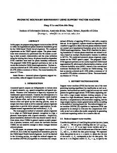
data completely, there is only one hyperplane with maximum margin. The hyperplane with maximum margin is less prone to noise and fluctuations of training data. So selecting this particular hyperplane wiIl correctly separate even noisy patterns and maximize prediction accuracy for previously unseen data. Let Xi be a vector in a vector space, a separating hyperplane is characterized with w xi -1 b=O In this formulation w is a vector orthogonal to the hyperplane and b is the bias term. As the figure 1 shows, for two-dimensional objects that belong to two classes (class +1 and class -1), the margin of optimum linear classifier is 2/11 W II. SO the wider margin is obtained by maximizing 2/11 W II which is equivalent to minimizing II w 112/2. ,

'

H ,

,

4. Experiments and results

,

w�'..t:,

,

+b

-"'1

=

+1 +1

Selecting the optimal parameters for SVM and MLP algorithms were done via k-fold cross validation technique. This approach avoids from overfitting the training examples and increases generalization accuracy over test data. In k-fold cross validation, our 150 training examples are partitioned into k subsets. In each fold, one subset is used for validation and the combination of the other subsets is used for training and the errors are then averaged. For the MLP algorithm, a three layers network structure with fourteen neurons in input layer (number of ear disorder symptoms) and one neuron in the output layer was configured. The number of neurons in hidden layer and the number of optimal iterations for training were determined via 6-fold cross validation. For this stage, in each fold, the number of iterations that satisfY at least one of the foIlowing two conditions on validation set is selected as the best, one is the sum of squared error (SSE) becomes lower than a desired error (supposed as 0.05 in our experiments) and the other is the difference between current epoch error and previous epoch error becomes greater than a predetermined threshold (supposed as 0.005 in our experiments). The second condition prevents from stopping training too soon when the validation set error begins to increase due to overfitting training examples [9]. After that, the mean of estimated iterations and their error rates are calculated. FinaIly the iteration mean is returned as optimal iteration and the error mean is returned as the error of cross validation (See table 3). As table 4 shows, the optimal node number in hidden layer is obtained 4 that yield the smaIlest cross validation error of 0.061 and respectively the optimal

+1

',1

+1

t1

+1 ,

,

,

Figure1. Separating hyperplane with maximum margin for two dimensional objects

SVMs can also be used to separate classes that cannot be separated with a linear classifier. In such cases, the coordinates of the objects are mapped into a high-dimensional feature space using kernel functions and thus they can be separated with a linear classifier. Finding the optimum separation hyperplane is a quadratic programming problem. Given training vectors Xi E Rn, i=1,.., 1 , in two classes and a vector yE Rnsuch that Yi E jl,-l}, C-SV classifier solves the foIlowing primal problem: I 1 T min-W W +C�>'i w,h,e 2 i=!

Yi (W1'(Xi)+ b)� 1- £i £i � 0, i=1,..., I.

Its dual is:

. 1 mm-a Ha-e a 2 O� Qi � C, i=l , ... ,1 LaiYi =0 i=! l'

l'

a

I

323

iteration is obtained 147 epochs. So a final run of back­ propagation is performed by training on all examples with the 4 nodes in hidden layer and 147 epochs. For the SVM method, some values for C and y parameters were chosen randomly. Then 10-fold cross validation was performed to select the best values of parameters. The optimal C and gamma are those that yield least cross validation error. Finally, training on whole training set was carried out using obtained optimal parameters. As table 5 shows, optimal parameters were found at C 48 and gamma 0.055, yielding the cross validation error of 0.014. After the training phase, the performance of two algorithms was evaluated using test data (previously unseen data). The result indicates that the MLP method diagnoses disorders with a 77.5% accuracy rate whereas the SVM algorithm has the accuracy of 92.5%. It can be seen that MLP does not work as well as SVM on the dataset with fourteen dimensionalities. Therefore, with using SVM model, the error rate can be decreased considerably and obtained more accurate classifier for classifying ear disorders. =

191

=

0.02

I.M. Corrigan, Patient Safety and Medication Errors, urI:

[I]

107'h Congress and Prescription Drug Safety, 200 I. [2] A.A. Bakars, Z. Othman, R. Ismail, Z.

Rough Set Theory for Mining the Level of Hearing Loss

0.098

International journal of computational Intelligence,

Estimated epoch 37

Cross validation error 0.107

4

147

0.061

5 7 10

191 115 21

0.098 0.108 0.152

of Technology Zakari, Using

Diagnosis Knowledge, International Conference on Electrical Engineering and Informatics, Malaysia,

[3]

2009.

S. Cox, M. Oakes, S. Wermter, M. Hawthorne, Medical

Data

Mining

in

Heterogeneous

Audiology

Records,

2004.

P. Thompson, X. Zhang, W. Jiang, Z.W. Ras, From

[4]

Mining Tinnitus Database To Tinnitus Decision-Support System,

IEEE/WIC/ACM

Intelligent Agent Technology,

validation

Neurons in hidden layer 3

[5]

S.

Moein,

M.H.

International

Conference

on

2007, pp. 203-207.

Saraee,

M.

Moein,

Iris

Disease

Classitying Using Neuro-Fuzzy Medical Diagnosis Machine, The

[6]

6th ISNN 2009, AISC 56, China, pp. 359-368.

O. Ivanciuc, Application of Support vector Machines in

Chemistry, Volume

Review

in

Computational

Chemistry,

23, pp. 291- 400.

2007,

[7] c.c. Chang, C.1. Lin, LIBSVM: A Library for Support

Vector Machines, http://www.csie.ntu.edu.tw/�cjlinllibsvrnl.

2009. [8] C.W. Hsu, C.C. Chang, C.l. Lin, A Practical Guide to Support Vector Classification,

C and gamma for

http://www.csie.ntu.edu.tw/�cj linll ibsvm/,

SVM via 10-fold cross validation

Gamma 0.01 0.1 0.5

0.014

0.06

http://nationalacademies.org/,

layer and epoch number via 6-fold cross

C 10 10 10

0.055

SSE 0.049 0.121 0.l31 0.049 0.061 0.179

Table4. Selecting optimal neurons in hidden

TableS. Selecting optimal

48

48

6. References

of MLP with S neurons in hidden

Average

0.02 0.027 0.02

The main contribution of this work was design of an accurate machine learning system for diagnosis six common ear disorders. Two popular machine learning methods were used, multi-layer perceptron neural network and support vector machine. The result showed that SVM achieved accuracy of 92.5% that is comparable to MLP with 77.5% accuracy. This shows that MLP does not work as well as SVM on high dimensional data. In the future, we are going to use a hybrid model for improving the performance of MLP algorithm on high dimensional data. Also applying machine learning algorithms to unknown problems would be interesting as the future works.

=

epoch 148 23 35 37 735 171

0.03 0.03 0.042

5. Conclusion

Table3. Estimating the optimal epoch number

fold 1 2 3 4 5 6

20 40 42

[9]

Cross validation error 0.054 0.02 0.027

Engineering! Math, ISBN:

324

2009.

T.M. Mitchell, Machine Learning, McGraw-Hili Science/

0070428077, 1997.