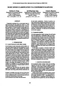
Abstractâ Bio-inspired robot swarms encompass a rich space of dynamics and collective behaviors. Given some agent mea- surements of a swarm at a ...
Classifying Swarm Behavior via Compressive Subspace Learning Matthew Berger,1 Lee M. Seversky,1 and Daniel S. Brown1
Abstract— Bio-inspired robot swarms encompass a rich space of dynamics and collective behaviors. Given some agent measurements of a swarm at a particular time instance, an important problem is the classification of the swarm behavior. This is challenging in practical scenarios where information from only a small number of agents may be available, resulting in limited agent samples for classification. Another challenge is recognizing emerging behavior: the prediction of swarm behavior prior to convergence of the attracting state. In this paper we address these challenges by modeling a swarm’s collective motion as a low-dimensional linear subspace. We illustrate that for both synthetic and real data, these behaviors manifest as low-dimensional subspaces, and that these subspaces are highly discriminative. We also show that these subspaces generalize well to predicting emerging behavior, highlighting that there exists low-dimensional structure in transient agent behavior. In order to learn distinct behavior subspaces, we extend previous work on subspace estimation and identification from missing data to that of compressive measurements, where compressive measurements arise due to agent positions scattered throughout the domain. We demonstrate improvement in performance over prior works with respect to limited agent samples over a wide range of agent models and scenarios.
I. INTRODUCTION Biological swarms are composed of many simple individuals following basic rules to form complex collective behaviors. Examples include flocks of birds, schools of fish, and colonies of bacteria, bees, and ants. The collective behaviors and movement patterns of swarms have long amazed observers, inspiring much recent research into designing bioinspired robotic swarms that use simple algorithms to collectively accomplish complex tasks [5], [16], [18]. Recently many researchers have tried to understand how to influence the collective behavior of a swarm using limited interactions [4], [10], [7], [22]; however, little work has looked at the reverse problem of trying to determine the collective behavior of a swarm from limited samples. In this paper we focus on the problem of classification of swarm behaviors. Identifying the specific behavior of a swarm is extremely useful for a number of applications. For example, in the robotics, controls, and human-factors communities, the specific collective state of a swarm may determine the best control policy to guide a swarm to a desired behavior. On the other hand, biologists may wish to classify the collective behavior of a school, flock, or herd as they track and evaluate how these biological swarms react to external stimuli. In particular, identifying emerging behavior or transient behavior, which leads to a specific form of behavior is very 1 Authors are with the Air Force Research Laboratory, Information Directorate
important for applications in swarm control, where we may want to ensure swarms exhibit certain forms of behavior and guide them away from other unwanted behaviors. Early detection and prediction of emerging collective behaviors are also important problems in observational biology, where scientists may want to determine exact causes for changes in collective behaviors [19], [12]. In many real-world situations, however, it is infeasible to assume that all members of a swarm are observable, posing significant challenges for classification. Many potential applications for swarms of robots include environments where limited and lossy communication may be the norm, such as exploring other planets, assessing and repairing damaged coral reefs, or locating tumors inside a human body. In these types of applications, it is unrealistic to assume that all of the robots can be observed at all times. Indeed, due to bandwidth constraints, occlusions, and noisy measurements it may be extremely difficult to get accurate information from even a small subset of the swarm. Thus, it is important to have methods for classifying and detecting collective behaviors that work well with limited samples. In this work, we cast swarm behavior classification from limited agent measurements as a problem of subspace identification. Our key observation is that many forms of swarm behavior dynamics, represented as collective agent motion, may be modeled as low-dimensional linear subspaces and that each behavior’s subspace is highly discriminative with respect to other behaviors. We also show that even for emerging behaviors, the transient dynamics are similarly lowdimensional and discriminative. Swarm identification thus can be reduced to identifying the subspace that the limited agent measurements most closely project onto. More specifically, we represent a single time instance of a swarm as a velocity field, where the collection of agent velocities are mapped to an underlying fixed resolution grid. A velocity field is identified as a point in a high dimensional space by associating each dimension with its unique grid location and vector coordinate, i.e. its x or y coordinate in 2D. This high dimensional space is the ambient space in which we seek to learn a subspace from a collection of vector fields. Note that we are faced with limited information even in learning a subspace for a given behavior, as it is highly unlikely for each grid location to map to a unique agent. To support agents positioned at arbitrary locations we treat the agent velocities as compressive measurements due to interpolation from the grid to each agent position. We extend previous work which handles subspace estimation from missing data [2] to this case of compressive measurements. We then leverage prior work on subspace detection from
compressive measurements [1] to robustly identify behavior types from just a few agent measurements. Our main contributions are summarized as follows: • We present a scalable and robust approach to learn discriminative behavior-specific subspaces from highly incomplete, compressive agent measurements. • Our approach is general with respect to different types of swarm behaviors. We assume that each behavior manifests as a discriminative low-dimensional subspace, compared to other approaches that use hand-engineered features or domain-specific classification techniques. • We obtain significant improvements in performance over the state-of-the-art in swarm classification, comprehensively demonstrated for different swarm models, agent sampling schemes, and for classifying both converged behavior and emerging behavior. II. RELATED WORK The limited-observation swarm classification problem was first proposed by Brown et al. [6]. Brown et al. examined swarm behavior classification for a model of robotic swarming which allows changes in the collective state of the swarm through limited interactions [7]. They show that a simple Naive Bayes classifier given limited samples from a swarm performs extremely well when trained on local features that directly relate to global collective features [6]. Brown et al. use a limited number of samples of agents’ turning rate and number of local neighbors to perform classification. This approach is computationally simple and works reasonably well even when only one agent can be sampled. However, they show that their model achieves only low to middling accuracy when there are transients in the behaviors. Another downside to this approach is that it requires hand-crafted features, limiting its applicability to swarm behaviors and data sets where this information may not be available. Recent work by Wagner et al. [21] investigated an alternative approach to swarm classification given limited observations that models a swarm as a Gaussian distribution over velocity fields and uses maximum likelihood estimations to impute unobserved entries of the velocity field. The benefits of this approach are that it provides a way to reconstruct a full velocity field based on a small number of observed agent’s positions and velocities. The downside is that this approach not only requires knowing the positions and velocities of every sampled agent, but also requires performing a Singular Value-based transformation to register the swarm onto a uniform grid. This transformation requires knowledge of the bounding box that encloses the entire swarm, including members of the swarm that are not assumed to be visible. Our approach is based on recent work in subspace estimation and identification from incomplete and more generally, compressive measurements. Balzano et al. [3] provided sample complexity bounds for reliably detecting whether an incomplete data vector belongs to a given subspace. The authors followed this by proposing a method for estimating a subspace from incomplete data, via a stochastic gradient descent technique restricted to the Grassmannian manifold,
termed GROUSE [2]. Other related approaches have been proposed to incorporate different regularization priors [15] to improve stability. Compressive measurements serve as a generalization to incomplete measurements, where there has been work on subspace detection from such data [1]. Krishnamurthy et al. [14] consider a similar compressive subspace learning problem as we do, however they assume that the original data is given and random projection operators may be generated to produce compressive measurements. In our approach, we are instead given compressive measurements, i.e. sampled agent velocities and define a compressive projection which interpolates the velocity field onto the agent positions. III. SUBSPACE MODELING OF SWARMS Our approach to swarm behavior identification is to first learn a subspace—per behavior type—from a set of characteristic fields of a swarm that collectively capture the dynamics of the swarm. In our work we take a swarm’s characteristic field as its velocity field defined over a regular grid of a fixed resolution, as in [21]. We make two key assumptions on the resulting subspaces: • Each subspace is low dimensional. This assumes that the collective motion of the agents associated with a swarm behavior are characterized by some lowdimensional dynamics. • The subspaces are discriminative with respect to each other. That is, when any given point on one subspace is projected into another subspace, its projection error is high. From these assumptions, a given swarm is then classified based on its velocity field’s projection into each subspace, taking the predicted subspace as that which gives the lowest projection error. The ambient space is a fixed resolution regular grid containing velocities of the swarm behavior. In practice, however, we are only given velocity vectors associated with agents scattered throughout the domain. This poses a major challenge—both for learning the subspace from training data and classifying behavior from a snapshot of a swarm at test time. In the following subsections, we detail our approaches for subspace learning and identification from collections of swarm velocities. A. Subspace Model Our approach learns a subspace from a collection of velocity fields for a given swarm behavior. We assume that we are given a collection of frames representing swarms— we make no assumptions on temporal coherency of swarms, we process all frames independently. The set of frames may arise from different simulations, different observation periods, etc.., yet we assume that collectively they form some underlying low-dimensional dynamics characteristic of the behavior. More specifically, assume that we have T frames of a swarm behavior, where the t’th frame has nt agents with positions Pt = {p1 , p2 , ..., pnt } and velocity vectors Vt = {v1 , v2 , ..., vnt }, where each pi , vi ∈ Rd . We first
map the agent positions Pt to a regular grid of a fixed resolution (s×s), where we map the minimum and maximum bounds of the agent positions at each frame to the minimum and maximum bounds of the grid. This is similar to the setup of [21], however, we do not attempt to find an affine transformation to compensate for distortion in the mapping. Instead, we assume the learned subspace will compensate for this distortion. The regular grid, of total dimension m = d · s2 , is the ambient space for our learned subspace. It represents the space of all possible vector fields for swarm frames. Our aim is to learn a linear subspace which spans all possible types of motion, modeled via agent velocities, for a given behavior type. However, each swarm frame contains velocities that are positioned at scattered points throughout the domain, hence standard subspace learning methods such as PCA are not appropriate, as we are not given velocities at the nodes of the grid. One possible solution to this problem is to interpolate the agent velocity vectors onto all grid nodes, and then perform subspace learning from the resulting dense field. However, the velocity vectors at grid nodes far away from all of the agent positions may not be well defined. To get around this, we may mark all such grid nodes as missing, and learn the subspace directly from these incomplete data vectors— the collection of grid nodes that contain interpolated velocity values, demonstrated in Figure 1(a). The method of GROUSE [2] has proven powerful for this problem of subspace estimation from incomplete data. GROUSE learns a subspace by performing stochastic gradient descent on the Grassmannian manifold—the space of all linear subspaces constrained to be orthogonal. They handle missing data by restricting subspace projections to observed values. In our scenario, we represent observed agent velocities for frame t sampled at mt grid nodes as a vector ˆft ∈ Rd·mt . Then for a given subspace U ∈ Rm×r of dimension r to be learned, GROUSE minimizes: F (U) = min kUΩt at − ˆft k22 at
T
s.t. U U = I,
(1)
where Ωt contains the mt indices corresponding to those grid nodes which have interpolated values corresponding to ˆft , and UΩ ∈ Rd·mt ×r subsamples the rows of U from Ωt . t A drawback to this approach, however, is that the subspace is learned from data that may fail to reflect the original agent velocities. In particular, for highly nonuniform data, the quality of the result can become highly dependent on the choice of interpolant, while for sparse data, an interpolant of local support may produce piecewise constant vectors in certain portions of the grid. More generally, it is nontrivial to determine the overall support of an interpolant—deciding on which grid nodes should be reported empty or not. B. Compressive Subspace Learning To circumvent these issues, we propose an approach which learns directly from the agent velocities ft by interpolating the subspace, rather than the given data. In a sense, this is
(a) Data Interpolation
(b) Subspace Interpolation
Fig. 1. Subspace learning with two different data models: (a) the subspace is learned from the field obtained by interpolating the input velocity vectors onto the grid, where in (b) we take a dual approach: the subspace is learned such that the subspace projection’s interpolation matches the input velocities. The latter is more faithful to the input data and less sensitive to highly sparse and nonuniformly distributed data.
dual to the scheme described above, where rather than interpolate the velocities onto the grid, we define an interpolant on the grid nodes for each individual agent velocity—see Figure 1(b). We first define ft ∈ Rd·nt , consisting of the nt agent velocities. We view ft as being drawn from a latent vector field defined on the regular grid gt ∈ Rm , where ft is formed by projecting gt onto the agent positions Pt via an interpolation matrix Wt ∈ Rd·nt ×m , i.e. ft = Wt gt . As in practice d·nt � m, we can interpret ft as a compressive measurement, with Wt as the compressive projection. Our goal is to learn a subspace from these compressive measurements, using the compressive projections taken as interpolants. Our approach extends GROUSE by defining the subspace projection with respect to the interpolation matrix, rather than a subsampling operator. This results in the following online formulation for a given swarm frame t: F (U) = min kWt Uat − ft k22 at
s.t.
UT U = I.
(2)
Here at is the subspace representation of ft which best fits the projection’s interpolation, found by a standard leastsquares solve. We seek a descent direction for U, via its gradient, which minimizes F while keeping us on the Grassmannian. Following the stochastic gradient descent protocol, the gradient of F follows as: ∇F = −2WtT (ft − Wt Uat )aTt .
(3)
A gradient step that preserves orthogonality is ultimately a function of the singular value decomposition (SVD) of ∇F . Similar to GROUSE, ∇F is rank one, hence its SVD has a simple form in terms of the residual vector r = WtT (ft − Wt Uat ), at , and its sole singular value σ = 2krkkat k. For a given step size ηi , the update is [2]: � � T 0 (cos(ηi σ) − 1) at r U =U+ Uat + sin(ηi σ) . kat k krk kat k (4) In practice, we first initialize U to be a random orthogonal matrix and then perform several passes over the swarm frames, updating U via the stochastic gradient step from
a single frame at a time. We use a decaying step size as suggested in [2], such that ηi ∝ 1i for the i’th iteration corresponding to a specific pass on a swarm frame. In all experiments we found that the subspace converged in at most five passes over the data. Regarding the interpolation matrix Wt , we simply use bilinear interpolation as highlighted in Figure 1(b), resulting in each row of Wt consisting of at most four nonzero entries. Hence, sparse matrix routines ensure that the algorithm can scale to very large data. Indeed, the overall complexity of the method is O(T mr), where r is usually very small—see Section IV-D for more details on setting r. Note that the previous work of [21] has complexity O(T m2 ). The original formulation of GROUSE is in fact a special case of our compressed formulation—if we assign each row of Wt a single 1 and 0 elsewhere, then Wt acts as a subsampling operator. One may also formulate this problem in terms of matrix completion with terms linear in X: argmin kXk∗ + X
T X
(Wt Xt − ft )2 ,
(5)
i=1
where Xt is a data column of X. One may then simply take the top left singular vectors of X as the subspace. However, matrix completion methods such as Singular Value Thresholding [8] do not scale well to the problem settings we consider for swarm identification, where m ∝ 104 and T ∝ 105 . Furthermore, we are not concerned with data imputation, we only require the subspace for identification. C. Swarm Classification via Subspace Identification At test time, given a set of swarm velocities at a frame f , classification is rather straightforward: we find the subspace in which the projection error of f is smallest, similarly to [1]. More formally, given f and its associated interpolation matrix W, its predicted behavior p(f ) is: p(f ) = argmin = i
k(I − PWUi )f k22 , kf k22
(6)
where I is the identity matrix, and PWUi is the compressed subspace projection operator, defined as PWUi = WUi (UTi WT WUi )−1 UTi WT . We divide by the squared norm of f to provide a normalized error, making the results interpretable for variably sampled agents. Different from [1], we do not transform W to be orthogonal, as it has no bearing on classification. There exists two remaining challenges we must address in classifying swarm behavior: handling a behavior whose subspace overlaps with other swarm behavior subspaces and determining bounds from subsampled agent measurements. 1) Classification via Projection Score Features: For certain types of swarm behaviors, their learned subspaces may intersect with other behavior subspaces, resulting in ambiguities for classification. Furthermore, other types of behaviors that are completely unstructured (i.e. agents moving randomly) may simply have a poorly fit subspace. To address both issues, we modify our classification scheme to treat each subspace projection score as a feature, and concatenate
(a) torus
(b) flock
(c) disordered
Fig. 2. Emergent swarm behaviors. Straight lines represent agent headings.
these scores as a feature space, from which we train a SVM to classify behaviors. Hence, a behavior whose projection error is low with respect to another behavior, but varies across other behaviors, will result in a discriminative feature. We can also classify the extreme case, a behavior that has high projection error on all subspaces, such as the disordered behavior shown in Figure 2(c). 2) Sliding Window Detection: An issue with limited agent information is that bounds of the agents may fail to match the original bounds of the full swarm data. The method of [21] assumes that the bounds for subsampled data are obtained from the original fully-sampled swarm data. In certain applications these bounds may be known a priori, i.e. due to environmental constraints, but in general this information may not be known. We propose a simple way to handle missing bounds by sliding an appropriate window over the subsampled agent’s domain, performing classification for each window, and taking the behavior which contains the strongest detection. We first compute behavior-specific mean bound sizes from training data swarm frames, using this as the expected bound size for the subsampled agents. A random window is generated by applying a transformation to the subsampled bounds such that the window size equals the expected bound size, while ensuring each agent is contained in the window. The strongest detection is determined via the highest SVM score, performed in a standard one-versus-all SVM classification. IV. EXPERIMENTAL SETUP In order to thoroughly test our subspace identification against previous approaches, we test across several different data models, subsampling schemes, and behavior types. We describe each of these components below. A. Swarm Datasets 1) Kerman Model: The Kerman model [13] consists of a set of agents following the dynamics x˙i = s · cos θi , y˙i = s · sin θi , θ˙i = ωi ,
(7)
where (xi (t), yi (t)) ∈ R2 is the ith agent’s position at time t, θi ∈ [−π, π] is the ith agent’s angular heading, s is the constant agent speed, and ωi is the ith agent’s angular velocity. Similar to Reynolds’ boids model [17], agents react to neighbors within an attraction, orientation, and repulsion zone. At each time step an agent’s neighbors are randomly chosen, where the probability of being neighbors is inversely proportional to the square of the distance between agents— yielding a simple model of occlusions and distance-limited
B. Subsampling Models We use two different types of agent subsampling schemes. We use uniform subsampling to select agents at random through the domain, simulating a random agent communication model, where only information from a subset of the swarm is available. This type of sampling was used in [6] to model unreliable or contested communication with a robot swarm. We also use a visibility-based subsampling model, similar to [21]. We associate each agent with a fixed radius, and designate a random position outside of the domain as an “observer”. Only agents which are seen by the observer are then taken as the samples, where an observer sees an agent if it is not occluded by any other agent. An agent is considered occluded if it has a neighbor that is closer to the observer and if a ray drawn from the observer to the agent in question intersects the “body” of the neighbor. We model each agent’s body by a disc centered at the agent’s position with the aforementioned radius. This tends to result in agents sampled near the boundary, only within the view of the outside observer, leading to very different sampling patterns from uniform sampling. C. Agent Behaviors We use two different types of agent behaviors in our experiments. One is considered converged, where the agents are definitively in one type of state, as determined by Tunstrøm’s order parameters criteria [19]. For the Kerman and Couzin model we take the end of the simulations as being converged, while for the fish data we take frames which are classified
1.0
1.0
torus flock
0.6
0.6
0.4
0.4
0.2 0.0
torus flock
0.8 normalized error
0.8 normalized error
sensing between agents. This model exhibits an interesting bi-stability—depending on the initial conditions, the simulation will converge to a stable flock or a stable torus with equal likelihood—see Figure 2. 2) Couzin Model: Couzin’s model [9] is similar to the Kerman model, but has several differences: it produces three possible group types: torus, flock, and disordered (see Figure 2); agents have a blind spot; agents react to neighbors within a maximum sensing range Ra ; and it adds explicit noise to the individual agent headings. These differences result in noisier behaviors that are more difficult to classify. 3) Golden Shiner Data: We obtained four data sets used by Tunstrøm et al. [19] to study collective states in schooling fish. This data was obtained by tracking groups of Golden Shiners in a broad shallow pool. The data includes each fish’s position and velocity. Despite the shallow depth, fish can still pass under one another. Due to these occlusions and tracking error, most frames have missing data. The four data sets correspond to schools of size 30, 70, 150, and 300 fish. Each school was filmed for 56 minutes at 30 frames per second. These schools of fish exhibit the three behaviors from Couzin’s model (disordered, torus, and flock) as well as transitory states as the school transitions between behaviors. 4) Labels: Each frame of the above data sets was labeled using the order parameter classification method described by Tunstrøm et al. that classifies swarm behaviors based on the alignment and rotation of the entire swarm [19].
0.2
1
3 5 7 subspace dimension
9
(a) Converged
0.0
1
3 5 7 subspace dimension
9
(b) Emerging
Fig. 3. Error plots depicting quality of subspace learning for the Kerman model for (a) swarm frames that have converged to their attracting behavior and (b) swarm frames that are emerging towards their attracting behavior.
as a certain type of behavior based on the frame’s order parameters. We also consider emerging behavior, wherein we would like to classify a transient swarm frame, based on the fact that we know which type of distinct behavior the agents will eventually form. We consider two types of experiments in this scenario: both training and testing on transient behavior, and training on converged behavior, while testing on transient behavior. The latter is especially challenging, as it tests to see how well a given classification method can generalize to unseen transient behavior. D. Implementation Details There are two main parameters to be set in our method: grid resolution and dimension of the subspace. The grid resolution needs to be large enough to faithfully interpolate the subspace to the given observations. This is a function of the ratio between the maximum and minimum distance between agent positions. We verified this distance ratio on the fish dataset, and found that a grid resolution of (64 × 64) adequately represented the data, hence for simplicity we used this resolution in all of our experiments. Since the Kerman and Couzin models contain repulsive forces, the minimum distance is lower bounded, and so this resolution is also suitable for these models. We found higher resolutions did not improve performance in our experiments. The subspace dimension should be large enough to capture variations in the swarms, yet small enough to still be discriminative with respect to other swarm behaviors. To better understand what the subspace dimensions should be, we trained our subspace on a converged set of frames for the Kerman model on flock and torus behaviors and analyzed the normalized projection error of the swarm frames as a function of dimension—see Figure 3(a). We observe that the subspace dimension for torus is 1 and for flock it is 2, up to the noise level in the data. This matches the intuition behind the different behaviors: velocity fields from a torus behavior are pointing in one direction or another, while flock behavior is unique up to a rotation, representing the additional dimension. Figure 4(a) visualizes the flock subspace via its spanning pair of vector fields. Note that any flock direction may be expressed as a linear combination of
0.011 0.0065 0.002
1.00
0.98 0.96 0.94 Subspace W-Subspace NB GP
0.92
(a) Converged Flock Subspace 0.90
2
3
4 5 6 7 8 9 number of samples
(a) Uniform Subsampling
10
classification accuracy
0.0155
1.00 classification accuracy
vector magnitude
0.02
0.95
0.90
0.85
0.80
Subspace W-Subspace NB GP
1.5 2.0 2.5 3.0 4.0 5.0 agent radius (% of bound diagonal)
(b) Visibility Subsampling
Fig. 5. Results for the Kerman swarm model for converged behavior across uniformly subsampled agents and visibility subsampled agents.
(b) Emerging Flock Subspace Fig. 4. Vector fields, visualized as flows via line integral convolution, which span the subspace for converged and emerging flock behavior.
does not assume bounds (W-Subspace). For each experiment we evaluate the methods on 10 train/test splits, reporting the mean behavior classification accuracy and standard deviation. A. Kerman Model
these fields. For generality across all data models, we have set the subspace dimensions for all convergent behaviors to 2 in all experiments. Transient swarm behavior prior to convergence to an attracting state is more nuanced: although agents are not moving in a defined behavior, there still exists structure in their motion. We observe this in Figure 3(b), where we show a similar experiment for determining the proper subspace dimension on the Kerman model for swarm frames sampled near the point of transition in the simulation: where transient behavior becomes either a torus or flock. We see that, although the subspace dimension is not as clear as the case of converging states, it still exhibits lowdimensional structure, roughly leveling off at a dimension of 3. Figure 4(b) visualizes the 3-dimensional subspace for Kerman flock behavior, where we can observe the original flock behavior augmented with smooth transitions to flock. In practice, we set the dimension to be 3 for emerging behavior in all of our experiments. V. RESULTS We compare our approach with the Naive Bayes method [6], denoted NB throughout, as well as the vector field Gaussian Process regression approach [21], denoted GP. NB was trained for the Kerman and Couzin models using turning rate and number of local neighbors as the features as detailed in [6]. We do not apply this classifier to the Golden Shiner since this data set does not include these features. To perform classification using GP we follow the methodology detailed in [21] to obtain reconstructed order parameters, where we set the grid resolution to (20 × 20)— larger resolutions were computationally prohibitive. Using Tunstrøm’s order parameter definitions of the disordered, torus, and flock, we label the frame as the behavior closest to the predicted order parameters. We present our approach for when the bounding box of the test swarm frame is known (Subspace), as well as the sliding window method which
We evaluate our approach on the Kerman model for converged and emerging behavior, across uniform and visibilitybased sampling. We used the same parameters as [6] to produce a flock or torus with approximately equal likelihood. We generated our data set by running 100 simulations starting from random initial conditions, resulting in 49 simulations that converged to a flock and 51 simulations that converged to a torus. Each simulation consists of 2000 frames for each behavior, giving enough time for the behaviors to fully emerge and stabilize. The converged behavior is taken to be the last 10% of each simulation, resulting in approximately 12000 frames for training and 8000 frames for testing, where we have verified that these frames correspond to their respectively consistent behavior according to [19]. We define emerging behavior to be frames sampled immediately before and after a transition point, unique for each simulation. The transition point is found as the last frame in the simulation which fails to be the particular behavior—i.e., every frame afterwards is consistently torus/flock as determined by the order parameter classification introduced by Tunstrøm [19]. Figure 5 shows the converged behavior on uniform sampling and visibility sampling. We find that our method consistently outperforms GP on both sampling schemes, highlighting that our approach is insensitive to the specific form of missing data. NB performs slightly better for very low uniform sampling rates, yet these particular experiments conform to their hand-engineered features quite well. Our sliding window method performs quite well, and usually has issues only for very small sampling rates (i.e. 2 agents). Table I shows the results for emerging behavior on uniform and visibility sampling. Compared to NB, our method performs much better when faced with visibility-subsampled data. Compared to GP we find that we are competitive, if slightly worse. We find that emerging behavior for the Kerman model can have large variation and our subspace model may not distinguish well between these variations. However, our comparable results come at a much lower
NB GP CS SW
Kerman Uniform Sampling 5 10 15 .82 ± .02 .85 ± .02 .87 ± .02 .85 ± .01 .87 ± .02 .88 ± .01 .84 ± .02 .87 ± .03 .88 ± .02 .81 ± .02 .85 ± .03 .86 ± .02
Kerman Visibility Sampling .03 .04 .05 .61 ± .01 .60 ± .01 .59 ± .01 .80 ± .02 .77 ± .02 .77 ± .01 .78 ± .02 .75 ± .02 .73 ± .01 .74 ± .02 .71 ± .03 .69 ± .01
Couzin Uniform Sampling 5 10 15 .63 ± .01 .69 ± .01 .72 ± .01 .83 ± .01 .90 ± 0.0 .93 ± .01 .82 ± .01 .90 ± .01 .93 ± .01 .81 ± .01 .90 ± .01 .93 ± .01
Couzin Visibility Sampling .03 .04 .05 .60 ± .02 .56 ± .02 .54 ± .03 .73 ± .01 .69 ± .01 .66 ± .01 .73 ± .01 .69 ± .01 .66 ± .01 .73 ± .01 .69 ± .01 .66 ± .01
TABLE I E MERGING BEHAVIOR RESULTS FOR THE K ERMAN AND C OUZIN MODELS . A LGORITHM NOTATIONS : NB [6], GP [21], CS IS OUR METHOD WITH KNOWN BOUND INFORMATION , AND SW IS OUR SUBSPACE - BASED SLIDING WINDOW CLASSIFICATION .
0.8 0.7 0.6
Subspace W-Subspace NB GP
0.5 0.4 2
3
4 5 6 7 8 9 number of samples
(a) Uniform Subsampling
10
0.9
Subspace W-Subspace NB GP
0.8 0.7 0.6
0.98
0.94 0.92 0.90 0.88 0.86 0.84 0.82
0.5
1.5 2.0 2.5 3.0 4.0 5.0 agent radius (% of bound diagonal)
(b) Visibility Subsampling
0.95
0.96
0.80
Subspace W-Subspace GP
5 6 7 8 9 10 11 12 13 14 15 number of samples
(a) Uniform Subsampling
classification accuracy
0.9
classification accuracy
classification accuracy
1.0
classification accuracy
1.0
0.90
Subspace W-Subspace GP
0.85 0.80 0.75 0.70 0.65
1.5 2.0 2.5 3.0 4.0 5.0 agent radius (% of bound diagonal)
(b) Visibility Subsampling
Fig. 6. Results for the Couzin swarm model for converged behavior across uniformly subsampled agents and visibility subsampled agents.
Fig. 7. Results for the Golden Shiner fish for converged behavior across uniformly subsampled and visibility subsampled agents.
average computational cost: our method takes approximately 7 seconds to train on the swarm frames, whereas GP takes approximately 500 seconds.
better than NB, we obtain very comparable results to GP. We note that compared to GP, our method achieves these results without resorting to domain-specific classification; furthermore the Window-Subspace method does not require knowledge of the entire swarm’s bounds. Hence, we see that the generality and ecological validity of our method does not come at the cost of lower performance.
B. Couzin Model Our Couzin model data set is generated with the same parameters used in [6] to reliably produce the model’s distinct behaviors. We generated 100 simulations each for flock, torus, and disordered behaviors. Each simulation starts from random initial conditions and consists of 1000 frames, giving enough time for each behavior to fully converge and stabilize, resulting in approximately 18000 frames for training and 12000 frames for testing. We use the same experimental protocol as the Kerman model for converging and emerging behavior, as well as uniform and visibility sampling, with the exception that for emerging behavior, we only test for flock or torus, as the disordered behavior fails to demonstrate transient behavior. Figure 6 shows results for converged behavior on uniform and visibility sampling. We find that our method greatly outperforms both methods across the different subsampling schemes. The Couzin model is quite noisy, yet we find that our method can both robustly learn subspaces, as well as reliably perform subspace projections for classification when faced with noisy and limited agent samples. GP performed rather poorly in classifying the disordered behavior, mainly due to a poor velocity field reconstruction, whereas we use the subspace projection error to determine that neither flock or torus is likely from the given data. Table I shows the results for emerging behavior on uniform and visibility sampling. Although our method performs much
C. Golden Shiner Data Last, we evaluate our method on the Golden Shiner fish dataset. Each frame of each dataset has its behavior labeled from [19], which we use to form the converging behavior experiments, using 10000 frames for training and 4000 frames for testing. For emerging behavior, here we wish to see if we can predict emerging behavior by only training on converged behavior in order to test the expressivity of our models. We fix the subsampling in these experiments (10 samples for uniform, radius of 2% of bound diagonal for visibility), and test on transient frames going backwards from the start of a converged state. In other words, we would like to see how early on we can predict where a transient behavior will eventually lead. Figures 7 and 8 show that our method consistently outperforms GP on all experiments. The sliding window technique mostly performs better, while assuming less information than GP. However, the gap in performance between Subspace and W-Subspace is larger compared with the synthetic datasets, as we found the nonuniformity in the fish positions to pose a larger challenge in the sliding window detection. Nevertheless, relative to GP, we find that our method performs quite well on the fish data in classifying emerging behavior
0.76
0.70
classification accuracy
0.72 0.70 0.68 0.66 0.64 0.62
Subspace W-Subspace GP
0.68 classification accuracy
Subspace W-Subspace GP
0.74
0.66 0.64 0.62 0.60 0.58 0.56
1
2
3 4 5 6 7 8 9 10 transients window size
(a) Uniform Subsampling
0.54
1
2
3 4 5 6 7 8 9 10 transients window size
(b) Visibility Subsampling
Fig. 8. Results for the Golden Shiner fish for emerging behavior. Here we fix the uniform subsampling to 10 frames and the agent radius (expressed as percentage of bounding box diagonal) to 2%, and vary the number of transient frames, going backwards from the start of converged frames.
compared to the Kerman and Couzin models, even with a more challenging train/test setup. The results on real data are highly encouraging, as they indicate the potential efficacy to be applied to collective motion patterns of actual robot swarms in the future. VI. CONCLUSIONS We have presented a method for swarm classification from partial data using subspace learning. We extend prior methods on subspace learning from incomplete information to that of compressive measurements, where we show that we are able to successfully learn subspaces from agent-based velocity fields, and classify swarms via subspace detection. Note the generality of our method—we do not perform data imputation, nor compute hand-engineered features at any stage of our approach. For future work, we would like to consider additional types of behavior models for classification. As our method is general, it should extend to arbitrary types of behaviors so long as each is driven by some underlying low-dimensional dynamics. For instance, the behaviors in [20] are modeled and parameterized via an ODE. We postulate that these degrees of freedom should manifest as such low-dimensional dynamics given observations of the agent velocities. We would also like to extend our formulation to detect outliers— agents which fail to adhere to the collective motion dynamics, modeled by the low-dimensional subspace. We note that our compressive subspace learning formulation uses an l2 norm in its energy, where by replacing it with a sparsityseeking l1 norm as in [11], our approach can be readily adapted to handle outliers, both in learning the subspace as well as classifying swarm behavior. R EFERENCES [1] M. Azizyan and A. Singh, “Subspace detection of high-dimensional vectors using compressive sampling,” in Statistical Signal Processing Workshop (SSP), 2012 IEEE. IEEE, 2012, pp. 724–727. [2] L. Balzano, R. Nowak, and B. Recht, “Online identification and tracking of subspaces from highly incomplete information,” in 48th Annual Allerton Conference on Communication, Control, and Computing (Allerton). IEEE, 2010, pp. 704–711.
[3] L. Balzano, B. Recht, and R. Nowak, “High-dimensional matched subspace detection when data are missing,” in International Symposium on Information Theory (ISIT). IEEE, 2010, pp. 1638–1642. [4] A. Becker, C. Ertel, and J. McLurkin, “Crowdsourcing swarm manipulation experiments: A massive online user study with large swarms of simple robots,” in Robotics and Automation (ICRA), 2014 IEEE International Conference on. IEEE, 2014, pp. 2825–2830. [5] M. Brambilla, E. Ferrante, M. Birattari, and M. Dorigo, “Swarm robotics: a review from the swarm engineering perspective,” Swarm Intelligence, vol. 7, no. 1, pp. 1–41, 2013. [6] D. S. Brown and M. A. Goodrich, “Limited bandwidth recognition of collective behaviors in bio-inspired swarms,” in Proceedings of the 2014 international conference on Autonomous agents and multiagent systems. International Foundation for Autonomous Agents and Multiagent Systems, 2014, pp. 405–412. [7] D. S. Brown, S. C. Kerman, and M. A. Goodrich, “Human-swarm interactions based on managing attractors,” in Proceedings of the 2014 ACM/IEEE international conference on Human-robot interaction. ACM, 2014, pp. 90–97. [8] J.-F. Cai, E. J. Cand`es, and Z. Shen, “A singular value thresholding algorithm for matrix completion,” SIAM Journal on Optimization, vol. 20, no. 4, pp. 1956–1982, 2010. [9] I. Couzin, J. Krause, R. James, G. Ruxton, and N. Franks, “Collective memory and spatial sorting in animal groups,” Journal of Theoretical Biology, vol. 218, no. 1, pp. 1–11, 2002. [10] E. Ferrante, A. E. Turgut, A. Stranieri, C. Pinciroli, M. Birattari, and M. Dorigo, “A self-adaptive communication strategy for flocking in stationary and non-stationary environments,” Natural Computing, vol. 13, no. 2, pp. 225–245, 2014. [11] J. He, L. Balzano, and A. Szlam, “Incremental gradient on the grassmannian for online foreground and background separation in subsampled video,” in Computer Vision and Pattern Recognition (CVPR), 2012 IEEE Conference on. IEEE, 2012, pp. 1568–1575. [12] Y. Katz, K. Tunstrøm, C. C. Ioannou, C. Huepe, and I. D. Couzin, “Inferring the structure and dynamics of interactions in schooling fish,” Proceedings of the National Academy of Sciences, vol. 108, no. 46, pp. 18 720–18 725, 2011. [13] S. Kerman, D. Brown, M. Goodrich, et al., “Supporting human interaction with robust robot swarms,” in 2012 5th International Symposium on Resilient Control Systems. IEEE, 2012, pp. 197–202. [14] A. Krishnamurthy, M. Azizyan, and A. Singh, “Subspace learning from extremely compressed measurements,” arXiv preprint arXiv:1404.0751, 2014. [15] M. Mardani, G. Mateos, and G. Giannakis, “Rank minimization for subspace tracking from incomplete data,” in 2013 IEEE International Conference on Acoustics, Speech and Signal Processing (ICASSP). IEEE, 2013, pp. 5681–5685. [16] R. Ramaithitima, M. Whitzer, S. Bhattacharya, and V. Kumar, “Sensor coverage robot swarms using local sensing without metric information,” in Robotics and Automation (ICRA), 2015 IEEE International Conference on. IEEE, 2015, pp. 3408–3415. [17] C. Reynolds, “Flocks, herds and schools: A distributed behavioral model,” in ACM SIGGRAPH Computer Graphics, vol. 21, no. 4. ACM, 1987, pp. 25–34. [18] M. Rubenstein, A. Cornejo, and R. Nagpal, “Programmable selfassembly in a thousand-robot swarm,” Science, vol. 345, no. 6198, pp. 795–799, 2014. [19] K. Tunstrøm, Y. Katz, C. C. Ioannou, C. Huepe, M. J. Lutz, and I. D. Couzin, “Collective states, multistability and transitional behavior in schooling fish,” PLoS Comput Biol, vol. 9, no. 2, p. e1002915, 2013. [20] G. Valentini, H. Hamann, and M. Dorigo, “Efficient decision-making in a self-organizing robot swarm: On the speed versus accuracy trade-off,” in Proceedings of the 2015 International Conference on Autonomous Agents and Multiagent Systems. International Foundation for Autonomous Agents and Multiagent Systems, 2015, pp. 1305– 1314. [21] G. Wagner and H. Choset, “Gaussian reconstruction of swarm behavior from partial data,” in 2015 IEEE International Conference on Robotics and Automation (ICRA). IEEE, 2015, pp. 5864–5870. [22] P. Walker, S. Amirpour Amraii, N. Chakraborty, M. Lewis, and K. Sycara, “Human control of robot swarms with dynamic leaders,” in Intelligent Robots and Systems (IROS 2014), 2014 IEEE/RSJ International Conference on. IEEE, 2014, pp. 1108–1113.