Imaging via Three-dimensional Compressive Sampling (3DCS)

Imaging via Three-dimensional Compressive Sampling (3DCS) ∗ Xianbiao Shu, Narendra Ahuja University of Illinois at Champaign-Urbana 405 N. Mathews Avenue, Urbana, IL 61801 USA {xshu2,n-ahuja}@illinis.edu

Abstract Compressive sampling (CS) aims at acquiring a signal at a sampling rate that is significantly below the Nyquist rate. Its main idea is that a signal can be decoded from incomplete linear measurements by seeking its sparsity in some domain. Despite the remarkable progress in the theory of CS, little headway has been made in the compressive imaging (CI) camera. In this paper, a three-dimensional compressive sampling (3DCS) approach is proposed to reduce the required sampling rate of the CI camera to a practical level. In 3DCS, a generic three-dimensional sparsity measure (3DSM) is presented, which decodes a video from incomplete samples by exploiting its 3D piecewise smoothness and temporal low-rank property. In addition, an efficient decoding algorithm is developed for this 3DSM with guaranteed convergence. The experimental results show that our 3DCS requires a much lower sampling rate than the existing CS methods without compromising recovery accuracy.

1. Introduction Digital images and videos are being acquired by new imaging sensors with ever increasing fidelity, resolution and frame rate. The theoretical foundation is the Nyquist sampling theorem, which states that the signal information is preserved if the underlying analog signal is uniformly sampled above the Nyquist rate, which is twice its highest analog frequency. Unfortunately, Nyquist sampling has two major shortcomings. First, acquisition of a high resolution image necessitates a large-size sensor. This may be infeasible or extremely expensive in infrared imaging. Second, the raw data acquired by Nyquist sampling is too large to acquire, encode and transmit in short time, especially in the applications of wireless sensor networks, high speed imaging cameras, magnetic resonance imaging (MRI) and etc. ∗ The support of the Office of Naval Research under grant N00014-091-0017 is gratefully acknowledged.

Compressive sensing [8, 4] or compressive sampling (CS), was developed to solve this problem effectively. It is advantageous over Nyquist sampling, because it can (1) relax the computational burden during sensing and encoding, and (2) acquire high resolution data using small sensors. Assume a vectorized image or signal x of size L is sparsely represented as x = Ψz, where z has K non-zero entries (called K-sparse) and Ψ is the wavelet transform. CS acquires a small number of incoherent linear projections b = Φx and decodes the sparse solution z = ΨT x as follows: min kzk1 z

s. t. Az , ΦΨz = Φx = b

(1)

where Φ is a random sampling (RS) ensemble or a circulant sampling ensemble. According to [5], CS is capable of recovering K-sparse signal z (with an overwhelming probability) from b of size M , provided that the number of random samples meets M ≥ αK log(L/K). The required sampling rate ( M L ), to incur lossless recovery, is roughly proportional to K L . A compressive imaging camera prototype using RS is presented in [9]. Recently, circulant sampling (CirS) [25]) was introduced to replace RS with the advantages of easy hardware implementation, memory efficiency and fast decoding. It has been shown that CirS is competitive with RS in terms of recovery accuracy [25]. CS often reduces the required sampling rate by seeking the sparsest representation or by exploring some prior knowledge of the signal. Image CS (called 2DCS) decodes each image independently by minimizing both its sparsity in wavelet domain and total variation (TV2D+2DWT) [15, 16]. However, due to the significant sparsity, the required sampling rate is still quite high. Video CS (called 3DCS) is introduced to further reduce the sampling rate by adding the temporal correlation. Adaptive methods sense a key frame by Nyquist sampling and then sense consecutive frames [23] or frame differences [26] by CS; Sequential methods first decode a key frame and then recover other frames based on motion estimation [13]. Joint methods recover a video by seeking its 3D wavelet sparsity (3DWT) [24], or by minimizing the wavelet sparsity of its first frame and subsequent

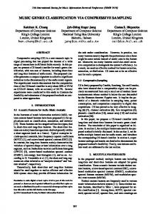
Figure 1. A compressive imaging (CI) camera using the proposed 3DCS. In this CI camera, a photographic lens (for forming image sequences, vectorized as It , 1 ≤ t ≤ T ) is followed by video compressive sampling, which consists of optical random convolution (C), random permutation (P ) and time-varying subsampling (St ) on a sensor. From the sampled data sequences Bt = St P CIt , 1 ≤ t ≤ T , the image sequences Iˆt , 1 ≤ t ≤ T is decoded by minimizing the 3DSM.

frame differences (Bk and Ck) [17]. However, none of the existing methods has exploited the major features of videos, i.e. 3D piecewise smoothness and temporal low-rank property. In this paper, a new 3DCS approach is proposed to facilitate a promising CI camera (Figure 1) requiring a very low sampling rate. Without any computational cost, this CI camera acquires the compressed data Bt , 1 ≤ t ≤ T , from which a video clip is recovered by minimizing a new 3D sparsity measure (3DSM). This 3DSM is motivated by two characteristics of videos. First, videos are often piecewise smooth in 2D image domain and temporal domain. Second, image sequences in a video are highly correlated along the temporal axis, which can be modeled as a temporal low-rank matrix [10] with sparse innovations. Thus, a new 3DSM is constructed by combining 3D total variation (TV3D) and the low-rank measure in the Ψ-transform domain (Psi3D). The contributions of this paper are as follows: 1. A generic 3D sparsity measure (3DSM) is proposed, which exploits the 3D piecewise smoothness and temporal low-rank property in video CS. Extensive experiments demonstrate (1) the superiority of our 3DSM over other measures in terms of much higher recovery accuracy and (2) robustness over small camera motion. 2. An efficient algorithm is developed for the 3DSM with guaranteed convergence, which enables the recovery of large-scale videos. 3. circulant sampling (CirS) is extended from 2DCS to video CirS, by adding time-varying subsampling. The 3DSM and its efficient decoding algorithm, together with the video CirS, constitute the framework of our 3DCS (Figure 1).

This paper is organized as follows. Section 2 presents the proposed 3DSM and video CirS. Section 3 develops the recovery algorithm for the 3DSM. Section 4 describes the experiments in comparison with existing methods. Section 5 gives the concluding remarks.

2. Proposed Method 2.1. Overview of our 3D sparsity measure (3DSM) In this section, a 3D sparsity measure (3DSM) is given for a fixed CI camera and will be extended to a moving camera later. A video clip is represented as a matrix I = [I1 , ..., It , ..., IT ], where each column It denotes one frame. For computational convenience, I is often vectorized as I = [I1 ; I2 ; ...; IT ]. A 3D sparsity measure (3DSM) is built by combining two complementary measures—3D total variation (TV3D) and 3D Ψ-transform sparsity (Psi3D). TV3D keeps the piecewise smoothness, while Psi3D retains the image sharpness and enforces the temporal low-rank property. As shown in Figure 1, the video I is recovered from the sampled data B by minimizing 3DSM. min TV3D(I) + γPsi3D(I) s. t. I

ΦI = B

(2)

where γ is a tuning parameter, Φ = diag(Φ1 , Φ2 , ..., ΦT ) is the video circulant sampling matrix, and B = [B1 ; B2 ; ...; BT ] is the sampled data.

2.2. 3D Total Variation In this section, TV3D is presented in detail. In 2DCS, total variation (TV) is often used to recover an image from incomplete measurements, by exploiting its piecewise smoothness in the spatial domain. The widely-used form of TV is TVL1L2 [15, 21, 16, 12], denoted as TV`1 `2 (It ) =

P p

(D1 It )2i + (D2 It )2i . In [22], the `1 -norm based TV measure TV`1 (It ) = kD1 It k1 + kD2 It k1 is proven to be better than TV`1 `2 in reducing the sampling rate. By extending TV`1 to the three-dimensional (spatial and temporal) domain, a new measure TV3D is formulated as:

2.4. Robustness over Camera Motion

i

TV3D(I) = kD1 Ik1 + kD2 Ik1 + ρkD3 Ik1

In this section, the 3DSM in Eq. (2) will be modified to be robust to camera motion. The 3DSM proposed in Eq. (2) explores the piecewise smoothness and the low-rank property, which is quite effective in improving the recovery accuracy of 3DCS. However, this model assumes a fixed camera or low-texture background. Even small camera motion might cause misalignments among real image sequences I = [I1 ; ...; IT ] and increase the temporal rank dramatically. these misalignments of I are modeled as a group of transformations (affine or perspective) Ω = {Ω1 , ..., ΩT } on well-aligned image sequences I˜ = [I˜1 ; ...; I˜T ] captured by a fixed camera. Specifically, It = I˜t ◦ Ωt , 1 ≤ t ≤ T . By introducing a group of transformations Ω, the 3DSM is extended to the moving camera as follows:

(3)

where (D1 , D2 , D3 ) are finite difference operators in 3D domain and ρ is proportional to the temporal correlation.

2.3. 3D Sparsity Measure in Ψ-transform Domain In a video captured by a fixed camera, most pixels correspond to static scene and almost keep constant value over time. This video is temporally correlated and sparsely innovated (a small number of pixels varies with time), the same as its Ψ-transform coefficients Z = [Z1 , ..., ZT ] = [ΨT I1 , ..., ΨT IT ]. Motivated by robust principal component analysis (RPCA) [3], Z is modeled as the sum of a low b Thus, Psi3D rank (LR) matrix Z and sparse innovation Z. is formulated as follows:

˜ + γPsi3D(I) ˜ s. t. ΦI = B, It = I˜t ◦ Ωt (7) min TV3D(I)

b 1 Psi3D(I) = min µRank(Z) + ηkZk1 + kZk b Z,Z

s.t.

T

Ψ I = Z + Zb

(4)

where Ψ = diag(Ψ, ..., Ψ), Z = [Z 1 ; ...; Z T ] and Zb = b The weight [Zb1 ; ...; ZbT ] are vectorized versions of Z and Z. coefficient µ tunes the rank of Z and η must be set as η ≤ 1; otherwise, the optimal Z is prone to vanish. Different from the RPCA which seeks Z and Zb from complete data b from incomplete I, our 3DCS needs to recover Z and Z projections B = ΦI. Thus, both the sparsity and rank of Z are explored to decode I. The proposed Psi3D attempts to minimize the number of nonzero singular values of Z, which is NP-hard and no efficient solution is known [7]. In practice, the widely P used alternative [6, 3] is the nuclear norm kZk∗ = k=1 σk (Z), which equals the sum of the singular values. Thus, the Psi3D is approximated as: b 1 Psi3D1 (I) = min µkZk∗ + ηkZk1 + kZk b Z,Z T b s.t. Ψ I = Z + Z

(5)

By assuming constant background, i.e., Rank(Z) = 1 and Z = [Z c , ..., Z c ], the Psi3D is simplified by deleting the rank term as follows: b 1 s.t. ΨT It = Z c + Z bt , ∀t (6) Psi3D2 (I) = ηT kZ c k1 + kZk By setting ηT = 1, the simplified Psi3D2 is similar to the joint sparsity model of multiple signals [1]. In the case of constant background, Psi3D2 requires less tuning parameters and computational cost than Psi3D1 . However, it is expected that Psi3D1 achieves higher recovery accuracy than Psi3D2 in the case of time-varying background (Rank(Z) > 1), e.g., illumination changes.

I,Ω

2.5. Video Circulant Sampling In this section, a video circulant sampling (CirS) is presented, which, together with a photographic lens, constitutes a compressive imaging camera (Figure 1). It consists of two steps: 1. Random convolution. Video CirS convolves an image It by a random kernel H, denoted by CIt , where C is a circulant matrix with H as its first column. C is b b is the diagonalized as C = F −1 diag(H)F, where H b = FH. It can Fourier transform of H, denoted by H be easily implemented using Fourier optics [20]. 2. Random subsampling, which consists of random permutation (P ) and time-varying subsampling (St ). St selects a block of M pixels from all N pixels on P CIt and obtains the data Bt = St P CIt , Φt It . Note that the selected block drifts with time t (Figure 1). To relax the burden of both sensing and encoding, it is desirable to implement a physical mapping from a random subset to a 2D array (sensor). Although it is challenging, a possible solution is to implement random permutation by a bundle of optical fibers, followed by a moving small sensor. The easy way—sensing the whole image CIt by a big sensor and throwing away the unwanted N − M pixels, does not benefit sensing but yields a method of computation-free encoding.

3. 3DCS Recovery Algorithms 3.1. 3DCS Recovery using Inexact ALM-ADM In this section, an efficient algorithm is presented to solve the 3DSM for a fixed camera. By introducing weight parameters α1 = α2 = 1, α3 = ρ, and auxiliary parameters

Algorithm 1 Solving 3DCS using inexact ALM-ADM b P , St and Bt , 1 ≤ t ≤ T Input: C, H, k+1 3 X Output: I b 1) αi kGi k1 + γ(µkZk∗ + ηkZk1 + kZk min 1: I 0 ← G0i ← b0i ← zeros(m, n, T ), 1 ≤ i ≤ 3; b I,Gi ,Z,Z 0 i=1 b0 ← d0 ← R0 ← g 0 ← zeros(m, n, T ). Z ←Z T b = Ψ I, Rt = CIt , St P Rt = Bt (8) 2: while I not converged do s.t. Gi = Di I, Z + Z b R} 3: Separate Rectification of: χ = {Gi , Z, Z, This linearly constrained problem can be solved by augk+1 k k χ ← arg minχ L(I , χ, λ ) mented Lagrangian multipliers (ALM) [12]. Given an L14: Joint Reconstruction: norm problem min kak1 s.t. a = b, its augmented La(I k+1 ) ← arg min L(I, χk+1 , λk ) grangian function (ALF) is defined as Lβ (a, b, y) = kak1 − 5: Update λ by “Adding back noise”: yβ(a − b) + β2 ka − bk22 . Then, the ALF of Eq. (8) is written bk+1 ← bki − τ (Gk+1 − Di I k+1 ) i i as T k+1 k k+1 d ← d − τ (Z − Ψ I k+1 ) 3 X k+1 k k+1 g ← g − τ (R − CI k+1 ) b R, bi , d, g) = αi Lβi (Gi , Di I, bi ) L(I, Gi , Z, Z, 6: k ←k+1 i=1 7: end while b 1 + β4 kZ + Zb − ΨT I − dk22 ) +γ(µkZk∗ + ηkZk1 + kZk 2 β5 2 + kR − CI − gk2 s.t. St P Rt = Bt , 1 ≤ t ≤ T (9) 3.1.1 Separate Rectification using Soft Shrinkage 2 where βi , 1 ≤ i ≤ 5 are over-regularization parameters, The convergence of the inexact ALM-ADM requires an λ , (b1 , b2 , b3 , d, g) is Lagrangian multipliers and C = exact solution to arg minχ L(I k , χ, λk ) at each iteration, diag(C, ..., C). ALM solves Eq. (8) by iterating between which can be obtained separately with respect to Gi , R b Define a soft shrinkage function as the following two steps: and the pair {Z, Z}. S(X, 1/β) = max{abs(X) − 1/β, 0} · sgn(X), where “·” 1. Solve (I k+1 , χk+1 ) ← arg min L(I, χ, λk ). denotes elementwise multiplication, then Gk+1 ,1 ≤ i ≤ 3 i 2. Update λk+1 with (λk , I k+1 , χk+1 ). are straightforwardly updated by b R), our 3DCS using Psi3D1 Eq. (2) can be χ , (Gi , Z, Z, rewritten as:

Each ALM iteration requires an exact minimization of b R), which is expensive. Fortunately, at fixed L(I, Gi , Z, Z, k b R) can be performed I and λ , minimization of L(Gi , Z, Z, independently. In this case, all the variables can be dib R}), and vided into two groups (I and χ = {Gi , Z, Z, k L(I , χ) can be minimized by applying the alternating direction method (ADM) [12]. Given λk+1 is updated at a sufficiently slow rate, the exact minimization can be simplified as only one round of alternating minimization (called inexact ADM). As shown in Algorithm 1, the inexact ALMADM solves our 3DCS by iterating among three major steps: (1) separate rectification of χ, (2) joint reconstruction of I and (3) update of λ. Given the exact solution to arg minχ L(I k , χ, λk ) is reached in the first step, the group of components χ is equivalent to a single variable and the inexact ALM-ADM with respect to two variables {χ, I} is guaranteed with convergence. Motivated by the convergence analysis in [11], the convergence condition of our recovery algorithm using inexact ALM-ADM is given as follows. Theorem 1 If the over-regularization parameters√ βi > 0, ∀1 ≤ i ≤ 5 and the step length τ ∈ (0, (1 + 5)/2), the video sequence I k+1 reconstructed by the inexact ALMADM (Algorithm 1) will uniquely converge the solution to Eq. (8).

Gk+1 ← S(Di I k + bki , i

1 ) βi

(10)

b are rectified from I k and dk by As for Psi3D1 , {Z, Z} singular value shrinkage (SVS)[2]. To meet the converb need be recgence condition in Theorem 1, the pair {Z, Z} tified iteratively until the pair is converged. In practice, the algorithm can be accelerated by just applying one round of rectification. k+1

← U S(Σ, µ/β4 )V T

k+1

k+1

Z Z

Zbk+1

← S(Z

(11)

, η/β4 )

T k

k

← S(Ψ I + d − Z

(12) k+1

, 1/β4 )

(13)

T where [U, Σ, V ] = svd(Ψ I k + dk − Zbk ). Similarly, as for b can be rectified without SVS operation. Psi3D2 , {Z, Z} The complete circulent samples R = [R1 ; ...; RT ] are rectified by 3D data I k and partial circulant samples Bt .

Rtk+1 Rtk+1 (Pickst , :)

← CItk

(14)

← Bt

(15)

where Pickst are the indices of rows selected by St .

3.1.2

Efficient Joint Reconstruction using 3D FFT

In this section, an efficient algorithm is presented to recover I k+1 jointly from rectified variables k+1 bk+1 , Rk+1 ). This algorithm is greatly (Gk+1 ,Z ,Z i accelerated by our 3DSM and video circulant sampling. By setting the derivative of L with respect to I to be zero, the optimal condition of I is induced as follows:

The main difficulty in solving Eq. (23) is the complicated dependence of aligned images I˜t = It Ωt on unknown transformations Ωt , 1 ≤ t ≤ T . It is almost impossible to solve I˜t and Ωt simultaneously. The ADM is applied to solve them by iterating between the following two steps:

1. Given Ωk , solve I k+1 ← minI F(I, Ωk ). This can be solved by adding forward and backward transformations in each iteration cycle of inexact ALM-ADM 3 X T T (Algorithm 1), however, it might be time-consuming. b αi βi Di (Gi − Di I − bi ) + γβ4 Ψ(Z + Z − Ψ I − d) To accelerate it, the misalignments Ωt are modeled as i=1 translation (∆xt , ∆yt ). According to Fourier shift theT (16) +β5 C (R − CI − g) = 0 orem, F(It ) is equal to multiplying F(I˜t ) by a linear ˆ· phase P (∆xt , ∆yt ). it is induced that CIt = F −1 (H Eq. (16)is reformulated into the form ΓI = Θ, where P3 −1 T ˆ ˜ ˜ F(It )) = F (H · P (∆xt , ∆yt ) · F(It )) = Ct I˜t , Γ = i=1 αi βi DiT Di +γβ4 +β5 C C. Under the periodic ˆ · P (∆xt , ∆yt )). Thus, I is rewhere C˜t = F −1 (H boundary condition [18] of finite operators Di , 1 ≤ i ≤ 3, ˜ followed by circulant shift T covered by fast solving I, both C C and DiT Di , 1 ≤ i ≤ 3 are block-circulant ma(∆xt , ∆yt ). trices. The operation Γ on 3D data I is equivalent to the sum of separate convolutions with five point spread functions PSFi , 1 ≤ i ≤ 5, which are given as follows: 3 X b 1) αi kGi k1 + γ(µkZk∗ + ηkZk1 + kZk min Horizontal: PSF = α β [1; −2; 1] (17) 1

1 1

I˜

= α2 β2 [1, −2, 1]

(18)

Temporal: PSF3

= α3 β3 [1 : −2 : 1]

(19)

Dirac delta: PSF4

= α4 β4 δ(x, y) ˆ ∗ · H) ˆ = β5 F −1 (H

(20)

Vertical: PSF2

2D: PSF5

(21)

where [A1 : A2 : A3 ] denotes concatenating A1 , A2 and ˆ ∗ is the complex A3 along the third (temporal) axis and H ˆ conjugate of H. According to the convolution theory, this optimal condition with respect to I can be solved efficiently by applying 3D fast Fourier transform. 5 X

F(PSFi ) · Ib = F(Θ)

(22)

i=1

where Ib = F(I). By defining the optical transfer funcP5 tion OTF , χk+1 and λk , Θk+1 can i=1 PSFi , given P3 k+1 k+1 T be updated as Θ = − bki ) + i=1 αi βi Di (Gi k+1 T bk+1 −dk )+β5 C (Rk+1 −g k ). Then, I k+1 +Z γβ4 Ψ(Z is recovered by applying inverse FFT the element-wise divisor of FΘk+1 by OTF. Our decoding algorithm is extremely efficient, for its joint reconstruction only requires two 3D FFT and some simple 1D/2D filtering.

3.2. 3DCS Recovery with Camera Motion

i=1

˜ Z + Zb = ΨT I, ˜ St P C˜t I˜t = Bt (24) s.t. Gi = Di I, 2. Given I k+1 , solve Ωk+1 ← minΩ F(I k+1 , Ω), without considering the constraint St P CIt = Bt . It is quite similar to robust image alignment. Readers are referred to [19] for detailed algorithms.

4. Experimental Results Although the compressive imaging camera has not been built, the 3DCS approach can still be evaluated by feeding the intermediate images It , 1 ≤ t ≤ T (Figure 1) with three surveillance videos from [14], i.e., an airport video (size: 144 × 176 pixels), a brighter lobby video (size: 128 × 160 pixels) and a darker lobby video (size: 128 × 160 pixels), as well as a video captured by a handheld camera (building video, size: 480 × 480). Our 3DSM (default: TV3D+Psi3D1 ) is compared with existing sparsity measures, such as TV2D+2DWT, 3DWT, Bk and Ck. Peak signal-to-noise ratio (PSNR) is used as the measure of recovery accuracy.

4.1. Parameter Selection

Assigning appropriate values to weight parameters γ, ρ, η, µ, τ and βi , 1 ≤ i ≤ 5 seems quite complicated but it is actually not. Weight parameters γ and ρ are often set to be greater than 1. η is often set to be T1 . µ depends on 3 X the rank of the background components in the video. Overb 1) F(I, Ω) = αi kGi k1 + γ(µkZk∗ + ηkZk1 + kZk regularization parameters βi , 1 ≤ i ≤ 5 prefer large vali=1 ues. To evaluate our 3DSM and its decoding algorithm, The T s.t. Gi = Di (I ◦ Ω−1 ), Z + Zb = Ψ (I ◦ Ω−1 ), St P CIt = Bt (23) values of the weight parameters are set empirically through In this section, the inexact ALM-ADM above can be adapted to solve Eq. (7) for the moving camera. The objective function can be relaxed as F(I, Ω) as:

all experiments, i.e. γ = 4, ρ = 3, η = βi = 100, ∀i.

1 T

, τ = 1.6 and

4.2. Evaluation of our 3DSM in video CS 4.2.1

Evaluation of 3DSM using Psi3D2

Figure 2. Recovery accuracy of different sparsity measures on a = 25%. 32-frame airport video at sampling rate M L

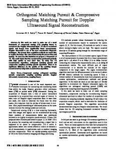
Figure 3. Averaged recovery accuracy of 10 frames at varying sampling rates in the brighter lobby video.

Fixed Sampling Rate. Our 3DSM is evaluated on the airport video (32 frames) at the sampling rate 25%, in comparison with other sparsity measures and a naive method— bicubic interpolation after half downsampling. The computing time is about 123 seconds on a normal computer (Intel E6320 CPU, 3 GB memory). As shown in Figure 2, our 3DSM achieves a recovery accuracy at least 6 dB higher than all the other methods at each frame. 2DCS fails to achieve high recovery accuracy, for the PSNR of its stateof-art (TV2D+2DWT) is lower than bicubic interpolation, which suffers from significant blur. As shown in Figure 4, our 3DSM recovery is much sharper, cleaner and closer to the original 4th frame. The recovery accuracy of our 3DSM decreases as the size of moving foreground grows, e.g., the 4th and 17th frames in Figure 4. Our 3DSM is tested on the brighter and darker lobby videos at the sampling rate of 30%. Figure 5 shows that our 3DSM decodes much better images (PSNR: up to 45 dB) than other measures and

the JPEG version of the original image (compression ratio: 30%). Our 3DSM achieves better recovery in the brighter lobby than that in the darker one, due to the significant photon-counting noise under the darker condition. Varying Sampling Rate. By varying the sampling rate, TV3D, Psi3D2 and 3DSM are tested on the brighter lobby video. As shown in Figure 3, either TV3D or our Psi3D is better (3 dB higher PSNR) than other measures at any sampling rate ( M L ), and their combination (3DSM) is better than each one alone. The superiority of our 3DSM over other M measures at M L = 25% is up to 7 dB. At L = 10%, 3DSM achieves the recovery accuracy (PSNR: 40 dB), which is conventionally considered to be lossless. Varying Video Size T . As shown in Figure 1, our 3DCS divides a video into short clips of T frames and then decode each short clip by minimizing our 3DSM. To study the influence of T on the decoding accuracy, a hybrid video is built by 16 frames from brighter lobby and 16 frames from from darker lobby. The average accuracy of all T frames using our 3DSM increases quickly with T in the beginning and reaches a stable value when T ≥ 10. When the lighting changes at the 17th frame, both the accuracy of Psi3D1 and that of Psi3D2 decrease to some extent (Figure 6). Psi3D1 and Psi3D2 . As shown in Figure 6, under constant lighting (T ≤ 16), our 3DSM using Psi3D2 is better than using Psi3D1 at any tuning parameter µ. However, under varying lighting conditions (T > 16), the decoding accuracy of Psi3D1 at µ = 100 remains almost invariant (46 dB ≤ PSNR ≤ 47 dB) as T increases, and is much higher than that of Psi3D2 . This can be explained by the background models of Psi3D1 and Psi3D2 . Psi3D1 uses a lowrank background model and can recover rank-2 background images (top row in Figure 7). Thus, the innovation images of Psi3D1 will be sparser than that of Psi3D2 , which rigidly assumes rank-1 background. Since the complete data I is unknown, the low-rank images recovered by Psi3D1 are different from the real background (Figure 7). Robustness over Motion. the robustness of our 3DSM over motion is evaluated by applying it to a video acquired by a moving (up and down) camera. As shown in Figure 8, without image alignment, our 3DSM can still recover the image sequences at M/L = 30% with acceptable accuracy (top row: PSNR > 31 dB). From this initial recovery, the transformations Ωt , 1 ≤ t ≤ 12 are estimated, of which the dominant components are translations (∆xt , ∆yt ). Given the translation knowledge, our 3DSM improves upon the initial recovery by 2.6 dB in terms of PSNR, less noise (e.g., bricks) and more detailed information (e.g., parking sign), as shown in Figure 8 (mid row). For computational efficiency, the translations are rounded to integer pixels. It is expected that our 3DSM recovery can be further improved by using perspective transformations.

(b) (f) (e) (a) (c) (d) Figure 4. Reconstructed images (top)of 4th frame and error maps at sampling rate M = 25% using (a) bicubic (PSNR: 24.42 dB), (b) L TV2D+2DWT (PSNR: 23.84 dB), (c) Ck (PSNR: 28.84 dB), (d) Bk (PSNR: 29.13 dB), and (e) our 3DSM (PSNR: 37.10 dB). (f) original 4th (top) and 17th (bottom) frames in airport video.

(a) (c) (d) (b) (e) (f) = 30% and error maps (bottom) from the bright video clip (10 frames) using (a) Ck (PSNR: Figure 5. Reconstructed images (top) at M L 40.62 dB), (b) Bk (PSNR: 39.75 dB) and (c) our 3DSM (PSNR: 46.09 dB), with (d) their original image (top) and error map of its JPEG version (bottom), compression ratio: 30%, PSNR: 40.59 dB). (d) Our 3DSM recovery (top, PSNR: 44.66 dB) and error map (bottom) from 30% circulant samples of the darker clip (10 frames), with (f) its original image (top) and error map of its JPEG version (bottom, compression ratio: 30%, PSNR: 42.53 dB).

Figure 6. Comparison of Psi3D1 and Psi3D2 by varying T . This hybrid lobby video consists of 16 frames from brighter lobby and 16 from the darker one.

5. Conclusion In this paper, a 3D compressive sampling (3DCS) approach has been proposed to facilitate a promising compressive imaging camera, which consists of video circulant sampling, 3D sparsity measure (3DSM) and an efficient decoding algorithm with convergence guarantee. By exploiting the 3D piecewise smoothness and temporal low rank property of videos, our 3DSM reduces the required sampling

(a) (b) (c) (d) Figure 7. Low rank recovery using our 3DSM (Psi3D1 , µ = 100) from the hybrid lobby video (brighter: 16 frames and darker: 16 frames) at M = 30%. Reconstructed 4 frames (bottom) with low L rank components (top): (a) (PSNR: 45.98 dB), (b) (PSNR: 46.36 dB), (c) (PSNR: 45.31 dB) and (d) (PSNR: 46.28 dB).

rate to a practical level (e.g. 10% in Figure 3). Extensive experiments have been conducted to show (1) the superiority of our 3DSM over existing sparsity measures in terms of recovery accuracy with respect to the sampling rate, and (2) robustness over small camera motion. Motivated by these exciting results, a real compressive imaging camera will be built, which is very promising for applications such as wireless camera network, infrared imaging, remote sensing and etc.

(a) (b) (c) Figure 8. Recovery of the 12-frame building video acquired by a handheld camera using our 3DSM at M/L = 30%. Top: initial results without image alignment (a) (PSNR: 31.50 dB), (b) (PSNR: 31.71 dB) and (c) (PSNR: 32.63 dB). From initial results, the estimated translations (∆x, ∆y) are listed as (a)(2.35, 3.11), (b) (0.62, -1.77), (c)(-0.31, 2.36). Middle: final results with estimated (∆x, ∆y) (a) (PSNR: 33.85 dB), (b) (PSNR: 34.10 dB) and (c) (PSNR: 35.18 dB). Bottom: three original frames.

References [1] D. Baron, M. B. Wakin, M. F. Duarte, S. Sarvotham, and R. G. Baraniuk. Distributed compressed sensing. Preprint. Available at www.dsp.rice.edu/cs., 2005. 3 [2] J. Cai, E. Candes, and Z. Shen. A singular value thresholding algorithm for matrix completion. preprint, 1984. 4 [3] E. Candes, X. Li, Y. Ma, and J. Wright. Robust principal component analysis? Journal of the ACM, 58(3):article 11, 2011. 3 [4] E. Candes, J. Romberg, and T. Tao. Stable signal recovery from incomplete and inaccurate measurements. Communications on Pure and Applied Mathematics, 59(8):1208–1223, 2006. 1 [5] E. Candes and T. Tao. Near-optimal signal recovery from random projections and universal encoding strategies? IEEE Transactions on Information Theory, 52(12):5406–5245, 2006. 1 [6] E. J. Candes and B. Recht. Exact matrix completion via convex optimization. Foundations of Computational Mathematics, 2009. 3 [7] A. L. Chistov and D. Y. Grigoriev. Complexity of quantifier elimination in the theory of algebraically closed fields. Mathematical Foundations of Computer Science, 176:17–31, 1984. 3 [8] D. Donoho. Compressed sensing. IEEE Transactions on Information Theory, 52(4):1289 – 1306, 2006. 1

[9] M. Duarte, M. Davenport, D. Takhar, J. Laska, and T. Sun. Single-pixel imaging via compressive sampling. IEEE Signal Processing Magazine, 25(2):83–91, 2008. 1 [10] C. Eckart and G. Young. The approximation of one matrix by another of lower rank. Psychometrika, 1(3):211–218, 1936. 2 [11] R. Glowinski. Numerical Methods for Nonlinear Variational Problems. Springer-Verlag, 1984. 4 [12] Y. Z. Junfeng Yang and W. Yin. A fast alternating direction method for tvl1-l2 signal reconstruction from partial fourier data. IEEE Journal of Selected Topics in Signal Processing, 4(2):288–297, 2010. 2, 4 [13] L. Kang and C. Lu. Distributed compressive video sensing. Proc. of International Conference on Acoustics, Speech, and Signal Processing, 2009. 1 [14] L. Li, W. Huang, I. Gu, and Q. Tian. Statistical modeling of complex backgrounds for foreground object detection. SIAM Journal on Scientific Computing, 13(11), 2004. 5 [15] M. Lustig, D. Donoho, J. Santos, and J. Pauly. Compressed sensing mri. IEEE Signal Processing Magazine, 25(2):72– 82, 2007. 1, 2 [16] S. Ma, W. Yin, Y. Zhang, and A. Chakraborty. An efficient algorithm for compressed mr imaging using total variation and wavelets. Proc. of IEEE Conference on Computer Vision and Pattern Recognition, 2008. 1, 2 [17] R. Marcia and R. Willett. Compressive coded aperture video reconstruction. Proc. of European Signal Processing Conference, 2008. 2 [18] M. K. Ng, R. H. Chan, and W. C. Tang. A fast algorithm for deblurring models with neumann boundary conditions. SIAM Journal on Scientific Computing, 21(3):851– 866, 2000. 5 [19] Y. Peng, A. Ganesh, J. Wright, and Y. Ma. Rasl: Robust alignment by sparse and low-rank decomposition for linearly correlated images. Proc. of IEEE conference on Computer Vision and Pattern Recognition, 2010. 5 [20] J. Romberg. Compressive sensing by random convolution. SIAM Journal on Imaging Science, 2009. 3 [21] J. K. Romberg. Variational methods for compressive sampling. SPIE, 6498:64980J–2–5, 2007. 2 [22] X. Shu and N. Ahuja. Hybrid compressive sampling via a new total variation tvl1. Proc. of European Conference on Computer Vision, 2010. 3 [23] V. Stankovic, L. Stankovic, and S. Cheng. Compressive video sampling. Proc. of European Signal Processing Conference, 2008. 1 [24] M. Wakin, J. Laska, M. Duarte, D. Baron, S. Sarvotham, D. Takhar, K. Kelly, and R. Baraniuk. Compressive imaging for video representation and coding. Proc. of Picture Coding Symposium, 2006. 1 [25] W. Yin, S. P. Morgan, J. Yang, and Y. Zhang. Practical compressive sensing with toeplitz and circulant matrices. Rice University CAAM Technical Report TR10-01, 2010. 1 [26] J. Zheng and E. L. Jacobs. Video compressive sensing using spatial domain sparsity. SPIE Optical Engineering, 48(8), 2009. 1