CLeVer: a Feature Subset Selection Technique for Multivariate Time ...

CLeVer: a Feature Subset Selection Technique for Multivariate Time Series? (Full Version) Kiyoung Yang, Hyunjin Yoon, and Cyrus Shahabi Computer Science Department University of Southern California Los Angeles, CA 90089, U.S.A. {kiyoungy,hjy,shahabi}@usc.edu

Abstract. Feature subset selection (FSS) is one of the techniques to preprocess the data before performing any data mining tasks, e.g., classification and clustering. FSS provides both cost-effective predictors and a better understanding of the underlying process that generated data. We propose a novel method of FSS for Multivariate Time Series (MTS) based on Common Principal Component Analysis, termed CLeVer. Traditional FSS techniques, such as Recursive Feature Elimination (RFE) and Fisher Criterion (FC), have been applied to MTS datasets, e.g., Electro Encephalogram (EEG) datasets. However, these techniques may lose the correlation information among features, while our proposed technique utilizes the properties of the principal component analysis to retain that information. In order to evaluate the effectiveness of our selected subset of features, we employ classification as the target data mining task. Our exhaustive sets of experiments show that CLeVer outperforms RFE and FC by up to 100% in terms of classification accuracy, while requiring significantly less processing time (up to 2 orders of magnitude) than RFE and FC. Keywords: Feature Subset Selection, Multivariate Time Series, Principal Component Analysis, Common Principal Component Analysis, Kmeans Clustering

1

Introduction

Feature subset selection (FSS) is one of the techniques to pre-precess the data before we perform any data mining tasks, e.g., classification and clustering. FSS is to identify a subset of original features from a given dataset while removing irrelevant and/or redundant features [1]. The objectives of FSS are [2]: – to improve the prediction performance of the predictors ?

A short version of this paper is to appear in the proceedings of the 9th Pacific-Asia Conference on Knowledge Discovery and Data Mining (PAKDD), Hanoi,Vietnam, 2005.

2

– to provide faster and more cost-effective predictors – to provide a better understanding of the underlying process that generated the data The FSS methods choose a subset of the original features to be used for the subsequent processes. Hence, only the data generated from those features need to be collected. The differences between feature extraction and FSS are: – Feature subset selection maintains information on the original features while this information is usually lost when feature extraction is used. – After identifying the subset of original features, only those features can be measured and collected ignoring all the other features. However, feature extraction in general requires measuring all the original features. A time series is a series of observations, xi (t); [i = 1, · · · , n; t = 1, · · · , m], made sequentially through time where i indexes the measurements made at each time point t [3]. It is called a univariate time series when n is equal to 1, and a multivariate time series (MTS) when n is equal to, or greater than 2. MTS datasets are common in various fields, such as in multimedia and medicine. For example, in multimedia, Cybergloves used in the Human and Computer Interface applications have around 20 sensors, each of which generates 50∼100 values in a second [4, 5]. In [6], 22 markers are spread over the human body to measure the movements of human parts while people are walking. The dataset collected is then used to recognize and identify the person by how he or she walks. In the Neuro-rehabilitation domain, kinematics datasets generated from sensors are collected and analyzed to evaluate the functional behavior (i.e., the movement of upper extremity) of post-stroke patients. The size of an MTS dataset can become very large quickly. For example, the EEG dataset in [7] utilizes tens of electrodes and the sampling rate is 256Hz. In order to process MTS datasets efficiently, it is therefore inevitable to preprocess the datasets to obtain the relevant subset of features which will be subsequently employed for further processing. In the field of Brain Computer Interfaces (BCIs), the selection of relevant features is considered absolutely necessary for the EEG dataset, since the neural correlates are not known in such detail [7]. An MTS item is naturally represented in an m × n matrix, where m is the number of observations and n is the number of variables, e.g., sensors. However, the state of the art feature subset selection techniques, such as Recursive Feature elimination (RFE) [2], require each item to be represented in one row. Consequently, to utilize these techniques on MTS datasets, each MTS item needs to be first transformed into one row or column vector. For example, in [7] where an EEG dataset with 39 channels is used, an autoregressive (AR) model of order 3 is utilized to represent each channel. Hence, each 39 channel EEG time series is transformed into a 117 dimensional vector. However, if each channel of EEG is considered separately, we will lose the correlation information among the variables.

3

In this paper, we propose a novel feature subset selection method for multivariate time series (MTS)1 based on common principal component analysis (CPCA) named CLeVer2 . In order to perform feature subset selection on an MTS dataset, CLeVer first obtains the descriptive common principal components (DCPCs) which agree most closely with the principal components of all the MTS items [8]. Note that the DCPC loadings represent how much each variable contributes to each of the DCPCs (See Section 2 for a brief review of PCA and DCPC). The intuition to use the DCPCs as a basis for variable subset selection is that they keep the most compact overview of the MTS items in a dramatically reduced space, while retaining both the correspondence to the original variables and the correlation among the variables. CLeVer subsequently clusters the DCPC loadings to identify the variables that have the similar contribution to each of the DCPCs. For each cluster, we obtain the centroid variable, eliminating all the similar variables within the cluster. These centroid variables form the selected subset of variables. Our experiments show that the performances of the variable subsets obtained by CLeVer perform up to about 100% better than other feature subset selection methods, such as Recursive Feature Elimination (RFE) and Fisher Criterion (FC) in terms of classification performance in most cases. Moreover, CLeVer takes up to 2 orders of magnitude less time than RFE, which is a wrapper method [9]. The remainder of this paper is organized as follows. Section 2 discusses the background. Our proposed method is described in Section 3, which is followed by the experiments and results in Section 4. Conclusions and future work are presented in Section 5.

2

Background

In this section, we briefly review principal component analysis and common principal component analysis. For more details, please refer to [10, 8]. 2.1

Principal Component Analysis

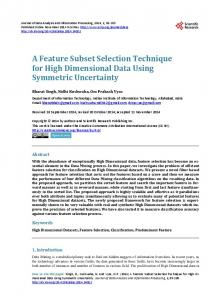
Principal Component Analysis (PCA) has been widely used for multivariate data analysis and dimension reduction [10]. Intuitively, PCA is a process to identify the directions, i.e., principal components (PCs), where the variances of scores (orthogonal projections of data points onto the directions) are maximized and the residual errors are minimized assuming the least square distance. These directions, in non-increasing order, explain the variations underlying original data points. That is, the first principal component describes the largest variation, the subsequent direction explains the next largest variance and so on. Figure 1(a) 1

2

For multivariate time series, each variable is regarded as a feature [7]. Hence, the terms feature and variable are interchangeably used throughout this paper, when there is no ambiguity. CLeVer is an abbreviation of descriptive Common principal component Loading based Variable subset selection method.

4 x2

PC 1_A PC 1_B CPC 1_AB

X2 PC 1 = (cos a 1 )X 1 + (cos ß 1 )X2

ß1

a1 X1

x1

PC 2

Score (Orthogonal Projection)

(a)

(b)

Fig. 1. (a) Two principal components obtained for one multivariate data with two variables X1 and X2 measured on 30 observations. (b) A common principal component of two multivariate data items with the same variables X1 and X2 measured on 20 and 30 observations respectively.

illustrates principal components obtained from a very simple (though unrealistic) multivariate data with only two variables (X1 , X2 ) measured on 30 observations. Geometrically, the principal component is a linear transformation of original variables. The coefficients defining this transformation are called loadings. For example, the first principal component (PC1) in Figure 1(a) can be described as a linear combination of original variables X1 and X2 , and the two coefficients (loadings) defining PC1 are the cosines of the angles between PC1 and variables X1 and X2 , respectively. In addition, the higher loading value of variable X2 implies that X2 is more dominant in the PC1 than X1 . The loadings are thus interpreted as the contributions or weights on determining the directions . 2.2

Common Principal Component Analysis

Common Principal Component Analysis (CPCA) is a generalization of PCA for N (≥ 2) multivariate data items, where the ith data item, (i = 1, . . . , N ), is represented in an mi ×n matrix [8, 11]. CPCA is based on the assumption that there exists a common subspace across all multivariate data items and this subspace should be spanned by the orthogonal components. One approach proposed in [8] obtained the Common Principal Components (CPC) by bisecting the angles between their principal components after each multivariate data item undergoes PCA. That is, firstly each of the multivariate data items is described by its first p principal components. Then, the CPCs are obtained by successively bisecting the angles between their jth (j = 1, . . . , p) principal components. These CPCs define the common subspace that agree most closely with every subspace of the multivariate data items. Figure 1(b) gives a plot of two multivariate data items

5

A and B. Let A and B be denoted as a swarm of white and black points, respectively, and have the same number of variables, i.e., X1 and X2 , measured on 20 and 30 observations, respectively. The first principal component of each dataset is obtained using PCA and the common component is obtained by bisecting the angle between those two first principal components. We will refer to this CPC model as Descriptive Common Principal Component (DCPC). Each common principal component loading for DCPCs, e.g., the (i, j)th element in a matrix that contains DCPCs, can be interpreted as the contribution of the jth original variable with respect to the ith common principal component, which is analogous to the way the principal component loadings are interpreted.

3

Proposed Method

We propose a novel variable subset selection method for multivariate time series (MTS) based on common principal component analysis (CPCA) named CLeVer. Figure 2 illustrates the entire process of CLeVer, which involves three phases: (1) principal components (PCs) computation per MTS item, (2) descriptive common principal components (DCPCs) computation per label3 and their concatenation, and (3) variable subset selection using DCPC loadings of variables. Each of these phases is described in the subsequent sections. Table 1 lists the notations used in the remainder of this paper, if not specified otherwise. Table 1. Notations used in this paper Symbol N n K p C |C|

3.1

Definition number of MTS items in an MTS dataset number of variables in an MTS item number of clusters for K-means clustering number of PCs for each MTS item to be used for computing DCPCs set of labels, i.e., {C1 , . . . , C|C| } number of unique labels

PC and DCPC Computations

The first and second phases (except the concatenation) of CLeVer are incorporated into Algorithm 1. It obtains both PCs and then DCPCs consecutively. The required input to Algorithm 1 is a set of MTS items with the same label. Though there are n PCs for each item, only the first p(< n) PCs, which are adequate for the purpose of representing each MTS item, are taken into 3

The MTS datasets considered in our analysis are composed of labeled MTS items. See Section 4.1 for details.

6 MTS Dataset V 1, … ,V n

V 1, … ,V n

Label A

Label B

I. Principal Components Computation PC 1 … PC p … PC n

II. Descriptive Common Principal Components Computation and Concatenation DCPC 1 … DCPC p

V 1, … ,V n

III. K-means Clustering on DCPC Loadings and Variable Selection

…

1

…

…

1

K

…

K

Selected Variables (one per cluster)

Fig. 2. The process of CLeVer.

consideration. It is commonplace that p is determined based on the ratio of the sum of the variances explained by the first p PCs to the total variance underlying the original MTS item, which exceeds, e.g., at least 0.8. Algorithm 1 takes the sum of variation, i.e., the threshold to determine p, as an input. That is, for each input MTS item, p is determined to be the minimum value such that the total variation explained by its first p PCs exceed the provided threshold δ for the first time (Lines 3∼10). Since the MTS items can have different values for p, p is finally determined as their maximum value (Line 11). All MTS items are now described by their first p principal components. Let them be denoted as Li (i = 1, . . . , N ). Then, the DCPCs that agree most closely with all PNN sets of p PCs are successively defined by the eigenvectors of the matrix H = i=1 LTi Li [8]: SV D(H) = SV D(

N X

LTi Li ) = V ΛV T

(1)

i=1

where rows of V T are eigenvectors of H and the first p of them define p DCP Cs for N MTS items. Λ is a diagonal matrix whose diagonal elements are the eigenvalues of H and describe the total discrepancy between DCPCs and PCs. For example, the first eigenvalue implies the overall closeness of the first DCPC to the first PC of every MTS item (for more details, please refer to [8]). This computation of DCPC is captured by Lines 16∼17.

7

Algorithm 1 ComputeDCP C: PC and DCPC Computations Require: MTS data groups with N items and δ {a predefined threshold} 1: DCP C ← ø; 2: H[0] ← ø; 3: for i=1 to N do 4: X ← the ith MTS item; 5: [U, S, U T ] ← SVD(correlation matrix of X); 6: loading[i] ← U T ; 7: variance ← diag(S); P 8: percentV ar ← 100 × (variance/ n j=1 variancej ); 9: pi ← number of the first p percentV ar elements whose cumulative sum ≥ δ; 10: end for 11: p ← max(p1 , p2 , . . . , pN ); 12: for i=1 to N do 13: L[i] ← the first p rows of loading[i]; 14: H[i] ← H[i − 1] + (L[i]T × L[i]); 15: end for 16: [V, S, V T ] ← SVD(H); 17: DCP C ← first p rows of V T ;

3.2

CLeVer

CLeVer utilizes a clustering method to group the similar variables together and select the least redundant variables, which is described in Algorithm 2. It takes MTS items and their label information as inputs. First, the DCPCs per label are computed by Algorithm 1 and are concatenated if the MTS dataset has more than 1 labels (Lines 3∼10). Subsequently, K-means clustering is performed on the columns of the concatenated DCPC loadings. That is, each column becomes one item for clustering. Hence, the column vectors with the similar pattern of contributions to each of the DCPCs will be clustered together. The intuition behind using the clustering technique for the variable selection is based on the observation that variables with similar pattern of loading values will be highly correlated and have high mutual information [12]. Since K-means clustering method can reach the local minima, we iterate the K-means clustering 20 times (Lines 11∼14). The next step is the actual variable selection, which involves deciding the representatives of clusters. Once the clustering is done, one column vector closest to the centroid vector of each cluster is chosen as the representative of that cluster. The other columns within each cluster therefore can be eliminated. Finally, the corresponding original variable to the selected column is identified, which will form the selected subset of variables with the least redundant and possibly the most related information for the given K.

8

Algorithm 2 CLeVer. Require: MTS data sets, |C| {the number of unique labels}, K {the number of clusters}, and δ {a predefined threshold} 1: Sbest ← ø; 2: DCP C ← ø; 3: if |C| ≤ 1 then 4: DCP C ← computeDCP C(MTS, δ); 5: else 6: for i=1 to |C| do 7: dc[i] ← computeDCP C(MTS with the label Ci , δ); 8: DCP C ← Concatenate(DCP C, dc[i]); 9: end for 10: end if 11: for i=1 to 20 do 12: (cnt[i], idx[i]) P ← Kmeans(DCP C loadings, K); 13: dist[i] ← K j=1 ED(cnt[j], items in the jth cluster); 14: end for 15: best ← min(dist[1], . . . , dist[K]); 16: (cntbest , idxbest ) ← (cnt[best], idx[best]); 17: Sbest ← extract K column vectors closest to cntbest of each cluster and identify the corresponding variables;

4

Performance Evaluation

We evaluate the effectiveness of CLeVer in terms of classification performance and processing time. We conducted several experiments on three real-world datasets. After obtaining a subset of variables using CLeVer, we performed classification using Support Vector Machine (SVM) with linear kernel. Subsequently, we compared the performance of CLeVer with those of Recursive Feature Elimination (RFE) [2], Fisher Criterion (FC), Exhaustive Search Selection (ESS), and using all the available variables (ALL). The algorithm of CLeVer for the experiments is implemented in M atlabT M . SVM classification is completed with LIBSVM [13]. 4.1

Datasets

The HumanGait dataset [6] has been used for identifying a person by recognizing his/her gait at a distance. In order to capture the gait data, a twelve-camera VICON system was utilized with 22 reflective markers attached to each subject. 15 subjects, which are the labels assigned to the dataset, participated in the experiments. The total number of data items is 540. Motor Behavior and Rehabilitation Laboratory, University of Southern California collected Brain and Behavior Correlates of Arm Rehabilitation (BCAR) kinematics dataset to study the effect of Constraint-Induced (CI) physical therapy on the post-stroke patients’ control of upper extremity [14]. The functional specific task performed by subjects was a continuous 3 phase

9

reach-grasp-place action. Four control (i.e., healthy) subjects and three poststroke subjects experiencing a different level of impairment participated in the experiments. The total number of data items is 39. The Brain Computer interface (BCI) dataset at the Max Planck Institute (MPI) [7] was collected to examine the relationship between the brain activity and the motor imagery, i.e., the imagination of limb movements. 39 electrodes were placed on the scalp to record the EEG signals at the rate of 256Hz. The total number of items is 2000, i.e., 400 items per subject. Table 2 shows the summary of the datasets used in the experiments. Table 2. Summary of datasets used in the experiments

# of variables average length # of labels # of items per label total # of items

4.2

HumanGait BCAR BCI MPI 66 11 39 133 454 1280 15 2 2 36 22/17 1000 540 39 2000

Classification Performance

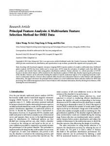
We first evaluated the effectiveness of CLeVer in terms of classification accuracy. Support Vector Machine (SVM) with linear kernel was adopted for the classifier. Using SVM, we performed leave-one-out cross validation for the BCAR dataset and 10 fold stratified cross validation [15] for the rest since they have too large number of items to conduct leave-one-out cross validation. For the MTS dataset to be fed into SVM, each of the MTS items should be represented as a vector with the same dimension, which we call vectorization. In [16], a correlation matrix is utilized to compute the similarity between two MTS items, which outperformed DTW and Euclidean distance with linear interpolation in terms of precision/recall. Hence, for CLeVer, Exhaustive Search Selection (ESS), and using all the variables (ALL), we vectorized each MTS item using the upper triangle of its correlation matrix. For RFE and FC, we vectorized each MTS item as in [7]. That is, each variable is represented as the autoregressive (AR) fit coefficients of order 3 using the forward backward linear prediction [17]. Therefore, each MTS item with n variables is represented in a vector of size n × 3. The The Spider [18] implementation of FC is subsequently employed. For small datasets, i.e., BCAR and HumanGait, RFE within The Spider [18] was employed, while for large dataset, i.e., BCI MPI, one of the LIBSVM tools [13] was modified and utilized. Note that ESS method was performed only on BCAR dataset due to the intractability of ESS for the large datasets. Figure 3(a) presents the generalization performances on the HumanGait dataset. The X axis is the number of selected subset of variables, i.e., the number

10 110 ALL

100 90

Precision (%)

80 70 60 50 40 30 20

CLeVer FC RFE

10 0

0

10

20

30 40 # of selected variables

50

60

70

(a)

(b)

110

100 ALL

100

90

MAX

90

80 70

70

Precision (%)

Precision (%)

80 AVG

60 50 40

10 2

3

40

4

5

6 7 8 # of selected variables

(c)

9

10

CLeVer FC RFE MIC 17 ALL

20

CLeVer RFE FC ESS

20

0

50

30

MIN

30

60

10 11

0

0

5

10

15 20 25 # of selected variables

30

35

40

(d)

Fig. 3. (a) Classification Evaluation for HumanGait dataset (b) 22 markers for the HumanGait dataset. The markers with a filled circle represent 16 markers from which the 27 variables are selected by CLeVer, which yields the same performance accuracy as using all the 66 variables. Classification Evaluations for (c) BCAR dataset and (d) BCI MPI dataset

of clusters K, and the Y axis is the classification accuracy. It shows that a subset of 27 variables selected by CLeVer out of 66 performs the same as the one using all the variables, which is 99.4% accuracy. The 27 variables selected by CLeVer are from only 16 markers (marked with a filled circle in Figure 3(b)) out of 22, which would mean that the values generated by the remaining 6 markers does not contribute much to the identification of the person. From this information we may be able to better understand the characteristics of the human walking. The performances by RFE and FC is much worse than the ones using CLeVer. Even when using all the variables, the classification accuracy is around 55%. Considering the fact that RFE on 3 AR coefficients performed well in [7], this may indicate that for the HumanGait dataset the correlation information among variables is more important than for the BCI MPI dataset. Hence, each variable should not be taken out separately to compute the autoregressive coefficients, by which the correlation information would be lost. Note that in [7], the order 3

11

for the autoregressive fit is identified after proper model selection experiments, which would mean that for the HumanGait dataset, the order of the autoregressive fit should be determined, again, after comparing different order models. This represents that it is not a trivial task to transform an MTS item into a vector, after which the traditional machine learning techniques, such as Support Vector Machine (SVM), can be applied. Figure 3(c) shows the classification performance of the selected variables on the BCAR dataset. The BCAR is the simplest dataset with 11 original variables and the number of MTS items is just 39. Hence, we applied the Exhaustive Search Selection (ESS) method to find all the possible variable combinations, for each of which we performed leave-one-out cross validation. The result of ESS shows that 100% classification accuracy can be achieved by no less than 6 variables out of 11. The dotted lines represent the best, the average, and the worst performance obtained by ESS, respectively. The result shows that CLeVer consistently outperforms RFE and Fisher methods. Figure 3(c) also depicts that the 7 variables selected by CLeVer produce about 100% classification accuracy, which is even better than using all the 11 variables which is represented as a horizontal solid line. This implies that CLeVer never eliminates useful information in its variable selection process. Figure 3(d) represents the performance comparison using the BCI MPI dataset 4 . It depicts that when the number of selected variables is less than 10, RFE performs better than CLeVer and FC technique. When the number of selected variables is greater than 10, however, CLeVer performs far better than RFE. The classification performance using the 17 motor imagery channels (MIC 17) is presented in dashed lines, while the performance using all the variables is shown in solid horizontal line. Using the 17 variables selected by CLeVer, the classification accuracy is 72.85%, which is very close to the performance of MIC 17 whose accuracy is 73.65%. Note again that even using all the variables, the performance of RFE is worse than that of 15 variables selected by CLeVer. 4.3

Processing Time

Table 3 summarizes the processing time of the 3 feature selection methods employed for the experiments. The processing time for CLeVer includes the time to perform Algorithm 1 and the average time to perform the clustering and obtain the variable subsets while varying K from 2 to the number of all variables for each dataset. For example, K changes from 2 to 66 for the HumanGait dataset. The processing time for RFE and FC includes the time to obtain 3 autoregressive fit coefficients and perform the feature subset selection. RFE is a wrapper feature selection method [15]. That is, RFE utilizes the classifier within the feature selection procedure to select the features which produce the best classification precision. Intuitively, CLeVer utilizes how much the 4

Unlike in [7] where they performed the feature subset selection per subject, the whole items from the 5 subjects were utilized in our experiments. Moreover, the regularization parameter Cs was estimated via 10 fold cross validation from the training datasets in [7], while we used the default value, which is 1.

12 Table 3. Comparison of processing time in seconds for different feature selection methods on 3 different datasets CLeVer RFE FC

HumanGait 6.2186 962.063 113.907

BCAR 0.2416 9.0390 6.4690

BCI MPI 48.0381 7886.844 7594.9413

variables contribute to the DCPCs in order to determine the importance and the similarity of them. Since CLeVer does not include the classification procedure, it takes less time to yield the feature subset than wrapper methods. For example, for the HumanGait dataset, CLeVer took less than 6 seconds to compute DCPCs, and a couple of seconds to perform K-means clustering on the loadings of the DCPCs. Overall, CLeVer take up to 2 orders of magnitude less time than RFE, while performing better than RFE up to about 100%.

5

Conclusion and Future Work

In this paper, we proposed a novel feature subset selection method for multivariate time series (MTS), based on common principal component analysis (CPCA), termed CLeVer. CLeVer utilizes the properties of the descriptive common principal components (DCPCs) to retain the correlation information among the variables. Subsequently, CLeVer performs clustering on the DCPCs loadings to select a subset of variables. Our experiments on the three real-world datasets show that CLeVer outperforms other feature selection methods, such as Recursive Feature Elimination (RFE) and Fisher Criterion (FC) in terms of classification performance. Moreover, CLeVer takes up to 2 orders of magnitude less processing time than RFE. We intend to extend this research in two directions. First, we plan to extend this work to be able to estimate the optimal number of variables, i.e., the optimal number of clusters K using, e.g., the Gap statistic [19]. We also plan to generalize this research and use k-way PCA [20] to perform PCA on a k-way array.

Acknowledgement This research has been funded in part by NSF grants EEC-9529152 (IMSC ERC), IIS-0238560 (PECASE) and IIS-0307908, and unrestricted cash gifts from Microsoft. Any opinions, findings, and conclusions or recommendations expressed in this material are those of the author(s) and do not necessarily reflect the views of the National Science Foundation. The authors would like to thank Dr. Carolee Winstein and Jarugool Tretiluxana for providing us the BCAR dataset and valuable feedbacks, and Thomas Navin Lal for providing us the BCI MPI dataset.

13

References 1. Liu, H., Yu, L., Dash, M., Motoda, H.: Active feature selection using classes. In: Pacific-Asia Conference on Knowledge Discovery and Data Mining. (2003) 2. Guyon, I., Elisseeff, A.: An introduction to variable and feature selection. Journal of Machine Learning Research 3 (2003) 1157–1182 3. Tucker, A., Swift, S., Liu, X.: Variable grouping in multivariate time series via correlation. IEEE Trans. on Systems, Man, and Cybernetics, Part B 31 (2001) 4. Kadous, M.W.: Temporal Classification: Extending the Classification Paradigm to Multivariate Time Series. PhD thesis, University of New South Wales (2002) 5. Shahabi, C.: AIMS: An immersidata management system. In: VLDB Biennial Conference on Innovative Data Systems Research. (2003) 6. Tanawongsuwan, Bobick: Performance analysis of time-distance gait parameters under different speeds. In: 4th International Conference on Audio- and Video Based Biometric Person Authentication, Guildford, UK (2003) 7. Lal, T.N., Schr¨ oder, M., Hinterberger, T., Weston, J., Bogdan, M., Birbaumer, N., Sch¨ olkopf, B.: Support vector channel selection in BCI. IEEE Trans. on Biomedical Engineering 51 (2004) 8. Krzanowski, W.: Between-groups comparison of principal components. Journal of the American Statistical Association 74 (1979) 9. Kohavi, R., John, G.H.: Wrappers for feature subset selection. Artificial Intelligence 97 (1997) 273–324 10. Jolliffe, I.T.: Principal Component Analysis. Springer (2002) 11. Flury, B.N.: Common principal components in k groups. Journal of the American Statistical Association 79 (1984) 892–898 12. Cohen, I., Tian, Q., Zhou, X.S., Huang, T.S.: Feature selection using principal feature analysis. University of Illinois at Urbana-Champaign (2002) 13. Chang, C.C., Lin, C.J.: Libsvm – a library for support vector machines. http://www.csie.ntu.edu.tw/∼cjlin/libsvm/ (2004) 14. Winstein, C., Tretriluxana, J.: Motor skill learning after rehabilitative therapy: Kinematics of a reach-grasp task. In: the Society For Neuroscience, San Diego, USA (2004) 15. Han, J., Kamber, M.: 3. In: Data Mining: Concepts and Techniques. Morgan Kaufmann (2000) 121 16. Yang, K., Shahabi, C.: A PCA-based similarity measure for multivariate time series. In: The Second ACM MMDB. (2004) 17. Moon, T.K., Stirling, W.C.: Mathematical Methods and Algorithms for Signal Processing. Prentice Hall (2000) 18. Weston, J., Elisseeff, A., BakIr, G., Sinz, F.: Spider: object-orientated machine learning library. http://www.kyb.tuebingen.mpg.de/bs/people/spider/ (2004) 19. Tibshirani, R., Walther, G., Hastie, T.: Estimating the number of clusters in a data set via the gap statistic. Journal of the Royal Statistical Society: Series B (Statistical Methodology) 63 (2001) 411–423 20. Leibovici, D., Sabatier, R.: A singular value decomposition of a k-way array for a principal component analysis of multiway data, pta-k. Linear Algebra and its Applications (1998)