Evolutionary Feature Subset Selection for Pattern Recognition

23 Evolutionary Feature Subset Selection for Pattern Recognition Applications G.A. Papakostas, D.E. Koulouriotis, A.S. Polydoros and V.D. Tourassis Democritus University of Thrace, Department of Production Engineering and Management Greece

1. Introduction A crucial part of a typical pattern recognition system is the extraction of the appropriate information that uniquely describes the patterns under processing. This information has the form of vectors and their contents are called features, which are constructed by specific extraction methods (Feature Extraction Methods - FEMs). The length of the extracted feature vectors may take high dimension by incorporating many features for each pattern, although this huge information may be redundant and in a lot of cases this extra information corrupts the separability of the patterns under recognition. Therefore the need of an additional pre-processing method that reduces the feature vectors’ dimension, by selecting the most appropriate features, subject to some performance indices (class separability, high classification error etc.) is necessary. This procedure is called dimensionality reduction or feature subset selection and has attracted the attention of the scientific community for the last thirty years (Molina et al., 2002). This chapter is focused on the usage of evolutionary methods in selecting the appropriate feature subset from a pool of features, in a way the resulted subset increases the recognition rates in several benchmark pattern recognition problems. A simple genetic algorithm is used to examine the usefulness of a predefined feature set of some benchmark problems from the literature and some useful conclusions about the ability of these features to recognize the patterns are drawn. Moreover, the dependency of the resulted feature subsets, as far as their classification abilities are concerned, on the form of the fitness function used to measure the appropriateness of the candidate solutions, constructed by the genetic algorithm, is studied in this chapter. Three fitness functions with different properties are examined and their performance is compared to each other, for a set of pattern recognition problems.

2. Feature subset selection Feature subset selection plays an important role in any pattern recognition system where the knowledge about the problem under consideration has to be modelled by appropriate data derived by the problem’s environment. Since these data may have very high dimension the presence of irrelevant or redundant information causes significant disorders in the whole recognition system.

444

Evolutionary Algorithms

First of all, the usage of massive data collections reduces significantly the training and evaluating performance of the mining or classifying stage of the recognition procedure. Therefore there is a need to keep these data as little as possible without loosing useful information about the problem to solve. On the other hand the presence of imprecise features can cause the misrepresentation of the knowledge which affects the generalization capabilities of the decision making module. From the above it is obvious that there is a need of a mechanism that analyses the entire data collection and forms the optimal feature subset, according to the following proposition, in terms of some performance indices. Proposition: A feature subset is called “optimal” if it has the lowest dimension that gives the highest recognition rate simultaneously. Many algorithms that attempt to find this optimal feature subset, in many disciplines, have been proposed in the past. Generally, there are three main categories (Liu & Yu, 2005) of feature selection methods: 1) wrapper (Talavera, 2005) methods, where a search mechanism evaluates candidate feature subsets by applying them to a specific classification model, 2) filter (Marono et al., 2007) methods, where the candidate subsets are evaluated without the presence of the mining model (they are independent of the classification model), instead the internal data properties/characteristics (dependency, correlation etc.) are measured and 3) hybrid (Das, 2001; Jashki et al., 2009) methods which make use of both filter and wrapper mechanisms by collaborating them in different steps. Ideally, an optimal subset has to be efficient, independent of the presence or not of the classification stage, since the internal characteristics of the features in a pool, determine their irrelevance and redundancy. However, due to the fact that a pattern recognition procedure constitutes a multi-step procedure, where its stage might affect each other, the operational behaviour of the classifying device (classifier) has to be considered. Therefore, while the filter methods are converged quite quickly, their resulted feature subsets may not work appropriately when applied on the classifier. On the other hand when wrapper methods are applied, the convergence to an optimal subset is slow and it highly depends on the structure of the classifier. A special case of feature selection methodologies are these methods which are making use of an evolutionary algorithm (Genetic Algorithms, Particle Swarm Intelligence, Evolutionary Strategies, etc.) as an optimization procedure with several different objective functions. Evolutionary feature subset selection has proved to be an effective selection tool, since the ability of the evolutionary algorithms to search in parallel many candidate solutions of the problem (Raymer et al., 2000; Papakostas et al. 2003, 2010; Uncu & Turkşen, 2007), guarantees their convergence to a near optimum solution subject to a performance index. In this chapter a Simple Genetic Algorithm (SGA), without having any advanced mechanism to prevent possible premature convergence to a problem solution is used, in order to optimize specific performance indices called objective functions. The presented algorithm is examined under three different configurations regarding the used objective function, the nature of which gives to the algorithm the characterization of filter or wrapper.

3. Genetic Algorithms (GAs) Genetic Algorithms (GAs) have played a major role in many applications of the engineering science, since they constitute a powerful tool for optimization. A simple genetic algorithm is

Evolutionary Feature Subset Selection for Pattern Recognition Applications

445

a stochastic method that performs searching in wide search spaces, depending on some probability values. For these reasons it has the ability to converge to the global minimum or maximum, depending on the specific application and to skip possible local minima or maxima, respectively. The main idea in which GAs are based, was first inspired by (Holland, 2001). He tried to find a method to mimic the evolutionary process that characterizes the evolution of living organisms. This theory is based on the mechanism qualified by the survival of the fittest individuals over a population. In fact, there are some specific procedures taking place until the predominance of the fittest individual. In the sequel, terminology in the field of genetic methods for optimization and searching purposes is given (Coley, 2001): • Individual (Chromosome) is a solution of a problem satisfying the constraints and demands of the system in which it belongs. • Population is a set of candidate solutions of the problem (chromosomes), which contains the final solution. • Fitness is a real number value that characterizes any solution and indicates how proper the solution for the problem under consideration is. • Selection is an operator applied to the current population, in a manner similar to the one of natural selection found in biological systems. The fitter individuals are promoted to the next population and poorer individuals are discarded. • Crossover is the second operator that follows the Selection. This operator allows solutions to exchange information, in the same way the living organisms use in order to reproduce themselves. Specifically two solutions are selected to exchange their substrings from a single point and after, according to a predefined probability Pc. The resulting offsprings carry some information from their parents. In this way new individuals are produced and new candidate solutions are tested in order to find the one that satisfies the appropriate objective. • Mutation is the third operator applied to an individual. According to this operation a single bit of an individual binary string can be flipped with respect to a predefined probability Pm. • Elitism is the procedure according to which, the fittest individual of each generation is ensured to be maintained in the next generation.

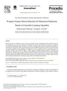
Fig. 1. Block diagram of a simple genetic algorithm.

446


After the application of these operators to the current population, a new population is formed and the generational counter is increased by one. This process will continue until a predefined number of generations is attained or some form of convergence criterion is met. A Simple Genetic Algorithm (SGA), which uses some of the operations discussed above, is presented in the above Fig.1. The usage of the SGA, depicted in Fig.1, in selecting the suitable feature subset for several benchmark datasets, for different objective functions is studied in the next section. 3.2 GA-based selection The most computational blocks of the above Fig.1 are independent of the application where the GA is applied. Only the coding/decoding of the population and the fitness calculation depend on the problem under solution. The application of the GA as feature subset selection algorithm involves the appropriate representation of the problem solution as chromosome structure of the algorithm’s population. Since the main goal of this work is to investigate the ability of each feature to describe the classes, the GA is repeatedly applied for all possible number of features from 1 to the maximum number. Therefore the algorithm’s chromosomes take variable length equal to the predefined number of features needed. In this way the general form of the m chromosomes of a population, where n features are searched, is as follows:

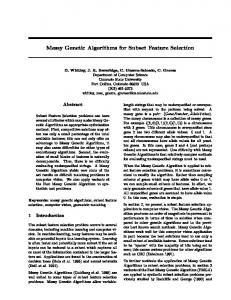
Fig. 2. Block diagram of chromosomes structure. In the above chromosome representation, n is equal to the number of the features being searched. For example, if the best 2 features are needed n is equal to 2 and each feature in the chromosome is labelled with a value (binary or real) lying inside the feature range of the pool. Moreover, appropriate handling to avoid multiple copies of the same feature to be included in the same chromosome, is required. The next processing stage, after the chromosome coding, is the determination of the objective (also defines the fitness of the candidate solutions) function, which is application dependent and constitutes the representation of the problem being optimized. The correct definition of the objective function is an important procedure since it has to fully describe the desired behaviour of the system. For pattern recognition purposes a simple objective function is the classification rate yielded when a set of features are selected. In order to compute the classification rate, a specific classifier is needed, so this version of GA-based selection belongs to the wrappers algorithms category. This first objective function has the following form: Objective Function #1

ObjFunc1 =

Number of incorrectly classified samples Total number of samples

(1)

447


The Minimum Distance classifier (Kuncheva, 2004) is used to compute the classification performance of the candidate feature subsets. This classifier operates by measuring the distance of each sample from the patterns that represent the classes’ centroid. The sample is decided to belong to the specific class having the less distance from its pattern. Since the performance of the classifier is highly dependent on the specific metric used to measure the distance of the samples from the classes, five well-known distances from the literature (Papakostas et al., 2010), the Euclidean, Logarithmic, Correlation Coefficient, Discrimination Cost and Hausdorff distancrs are selected and presented in the following: Euclidean Distance Logarithmic Magnitude Distance

d1 ( p , s ) =

n

∑ ( pi − si )

(2)

i =1

n

∑ ( log pi

d2 ( p , s ) =

2

i =1

− log si

)

2

(3)

n

Correlation Coefficient

d3 ( p , s ) =

∑ pi si

n

∑ ( pi )

2

i =1

Discrimination Cost Function

Hausdorff Distance

i =1 1/2

n

∑ ( si )

2

1/2

i =1

n ⎡ max ( p , s ) ⎤ vi ki d4 ( p , s ) = ∑ ⎢ − 1⎥ min p , s ( ) i =1 ⎣ ⎢ vi ki ⎦⎥

2

d5 ( p , s ) = max ( h ( p , s ) , h ( s , p ) ) h ( p , s ) = max min p − s p∈p

(4)

(5)

(6)

s∈s

The above formulas measure the distance between two vectors p = [ p1 , p2 , p3 ,..., pn ] s = [ s1 , s2 , s3 ,..., sn ] , which are defined in the \ n space. It has to be remarked that the above measures tend to 0 for the case of two equal vectors, except d3 which gives 1, since it counts the similarity of the two vectors. Finally, when the GA-based feature selection method is used, these measures are treated as objective functions aimed to being minimized (d1, d2, d4, d5) or maximized (d3). Noted that a maximization problem can be transformed to a minimization one, by minimizing the opposite objective function (-F instead F). The second examined objective function describes the internal relationships of the feature vectors describing each class and is based on the Pearson Correlation Coefficient (Wikipedia). This function measures the within-class and between-class correlation of the feature vectors belonging to the same class and the feature vectors of different classes respectively. In a similar way as in the case of Fisher Criterion, the objective is the maximization of the following quantity. Objective Function #2

ObjFunc 2 =

rw rb

(7)

448


where rw is the within-class Pearson correlation coefficient defined as Within-class correlation

rw =

1

C max

C max

c =1

∑

rc

(8)

with rc = ri ,c =

1 Nc

Nc

(9a)

∑ ri ,c

i =1

Nc 1 rij ∑ N c − 1 j = 1,i ≠ j

(9b)

and rb is the between-class Pearson correlation coefficient defined as Between-class correlation

rb =

C max C max

1

(C max − 1 )

2

∑ ∑

i = 1 j = 1, i ≠ j

ri j

(10)

with rcd =

1 Nd d ∑ ri ,c N d i =1

rid,c =

1 Nc

(11a)

Nc

∑ rij

j =1

(11b)

In the above equations (8)-(11), Cmax is the number of classes and NC the number of samples belonging to the class C. The maximization of the ObjFunc2, indicate the existence of the appropriate feature vectors which guarantee high correlation between the vectors that describe the same class and low correlation between the vectors of different classes. The GA-based selection procedure which uses the function defined in (7) as the objective being optimized, constitutes a filter selection method, since it is independent from the classifier device used to take the final decision. The third objective function which is studied in this investigation, is a hybrid function formed by the combination of the previous two functions ObjFunc1 and ObjFunc2, according to the following weighted combination rule. Objective Function #3

ObjFunc 1 = w1 × ObjFunc 1 + w2 × ObjFunc 2

(12)

where the weights w1 and w2, controls the importance of each objective function regarding their ability to describe the problem under process. The definition of (12) corresponds to a generalized formula of an objective function, where the functions of (1) and (7) are special cases derived from (12), by setting w2=0 and w1=0, respectively. Although, a separate study on the appropriate selection of the w1, w2 weights is needed in order to improve the overall feature selection procedure, the same value of 0.5 is selected for the experiments, by giving the same degree of importance to the two objective functions.

449


It is important to notice that the GA-based selection scheme has the advantage to permit the usage of non differentiable functions as objective functions, in contrast to the gradient-based optimization methodologies working only with differentiable error functions.

4. Experimental study For experimental purposes, several well-known benchmark datasets from the pattern classification research field are selected, where the usefulness of their default number of features are examined, according to the GA-based selection schemes presented in the previous section. The experimental benchmarks are widely used in the literature and are selected from the UCI repository (UCI-Machine Learning Repository), with their properties being summarized in the following Table 1.

Dataset Iris Wine Pima Indians Diabetes Thyroid Parkinson Hepatitis Glass

Features 4 13 8 5 22 19 9

Instances 150 178 768 215 195 155 214

Classes 3 3 2 3 2 2 6

Table 1. Properties of benchmark datasets. In all the experiments the GA operates with the configuration shown in Table 2, although each classification problem needs its own configuration in order to achieve the best performance. However, this common GA configuration does not affect significantly the selection procedure, since even taking into account a suboptimal solution, significant conclusions can be drawn, which can further be improved by appropriate algorithm’s calibration.

Parameter Population Size Variables Range Maximum Generations Elitism Crossover Points Crossover Probability Mutation Probability Selection Method

Value 10 [1,n] n: number of features 100 YES, 2 chromosomes 2 points 0.8 0.001 Uniform Selection

Table 2. Simple Genetic Algorithm settings. Three feature selection experiments are arranged, where the GA optimization scheme used to select the best features by using the three objective functions defined in (1), (7) and (12). For a predefined desired number of features, the algorithm returns the best features’ combination for each one of the datasets and the corresponding formed vectors are presented in the following sections.

450

Evolutionary Algorithms st

4.1 Experiment 1 – 1 objective function (a wrapper case) In the first experiment the objective function of equation (1) is applied, as a fitness measure of each candidate feature subset, while the five metric distances (2)-(6) is used as minimum distance classification module. Since the first objective function measures the classification performance of the candidates feature subsets, there is a need to define the representative patterns that best characterize the classes’ distributions in each benchmark problem. These patterns correspond to the classes’ centers and are decided by taking into account a specific part of the entire dataset, called training set. In fact three different data collections are used in this experiment, the 25%, 50% and 75% randomly selected samples of each dataset, while the rest samples, called testing set, in each case are used for evaluation purposes. Moreover, each execution of the GA-based selection has been repeated 10 times in order to extract more statistically corrected results and the corresponding mean values are summarized in the following Tables (3)-(9) (for the case of 50% training data samples).

Metric Best Feature Subset Objective Value All Features Objective Value

Iris Dataset d2

d1 3,4 0.973

1,4 0.973

d3 4 0.960

d4 1,4 0.973

d5 3,4 0.973

0.893

0.973

0.866

0.973

0.893

Table 3. Selection results for the Iris dataset.


Wine Dataset d2 d3 3,4,5,7,10,11, 2,6,7,10,12 1,2,3,7,9,10,12 12,13

d4 1,3,4,5,7,10, 11,12,13

0.933

0.988

0.900

0.988

0.933

0.700

0.933

0.711

0.933

0.700

d1

d5 1,2,3,7,9,10,12

Table 4. Selection results for the Wine dataset.


Pima Indians Diabetes Dataset d1 d2 d3 1,3,5,7 1,5,7 1,7 0.750 0.760 0.742

d4 1,5,7 0.763

d5 1,3,5,7 0.750

0.679

0.554

0.679

0.555

0.713

Table 5. Selection results for the Pima Indians Diabetes dataset.

451



2,3 0.906

Thyroid Dataset d2 d3 2,3,4 3,4,5 0.943 0.915

d4 2,3,4 0.943

d5 2,3 0.906

0.850

0.846

0.887

0.850

d4 1,16,21,22 0.855

d5 17,20,22 0.855

0.690

0.721

d1

0.710

Table 6. Selection results for the Thyroid dataset.


d1 17,20,22 0.855 0.721

Parkinson Dataset d2 d3 1,16,21,22 17,20,22 0.855 0.855 0.690

0.701

Table 7. Selection results for the Parkinson dataset.


d1

Hepatitis Dataset d2 d3

d4

d5

5,10,12,14,17,19

1,10,12

2,12,13,14

1,3,12

3,5,10,12,14,17,19

0.870

0.860

0.870

0.860

0.870

0.545

0.652

0.584

0.652

0.545

Table 8. Selection results for the Hepatitis dataset.


d1 2,4,8,9 0.458

Glass Dataset d2 d3 2,4,7 2,3,4,7,8 0.458 0.440

d4 2,4,7 0.458

d5 2,4,8,9 0.458

0.403

0.247

0.247

0.403

0.357

Table 9. Selection results for the Glass dataset. An important conclusion is drawn from the above tables, about the usefulness and information redundancy of the nominal features describing all the benchmark datasets. In all the cases there is a feature vector with lower dimension and higher objective value than the corresponding vectors consisting of all the features. This means that the classification performance can be significantly improved by using a small feature subset, while the usage of all the features does not guarantee better classification results. Therefore, by applying a classification-driven dimensionality reduction mechanism based on GA selection scheme, only the most essential features are kept. Moreover, the above tables show the ability of each metric distance (d1)-(d5) to measure the real distance between the data points and the corresponding classes’ centers. Due to the fact that none of the above distance shows significant superior performance over the rest ones, an additional statistical analysis, which counts the frequency of the features including in the best feature subsets for all distances and training sets (25%,50%,70%), is applied and the resulted histograms are illustrated in the following Fig.3.

452


(a)

(b)

(c)

(d)

(e)

(f)

453


(g) Fig. 3. Features histograms for (a) Iris, (b) Wine, (c) Pima Indians Diabetes, (d) Thyroid, (e) Parkinson, (f) Hepatitis and (g) Glass datasets. By analysing the above plots of Fig.3, the suitability of each feature in the case of all datasets, can be studied. Through these plots, the statistically most efficient feature subsets for all metric distances are constructed, as a supplementary to the GA-based feature selection mechanism. The final features subsets for each dataset are summarized in the following Table 10. It has to be noted that the usefulness of these features subsets will be studied later by using them to solve the same pattern recognition problems, with a typical feedforward neural network classifier used as the decision module.

Datasets Iris Best Feature 3,4 Subset

Wine

Pima Indians Thyroid Diabetes

1,2,3,6,7,10, 1,3,5,7 11,13

2,3,4

Parkinson

Hepatitis

Glass

1,2,3,9,10,13, 1,2,3,4,5,7,9, 14,16,17,18,19, 10,11,12,13,14, 2,4,7,8 20,21,22 17,19

Table 10. Resulted feature subsets from the analysis of the histograms of Fig.3. 4.2 Experiment 2 – 2nd objective function (a filter case) The only difference between the 2nd experiment and the 1st one is the usage of a different objective function for the evaluation of the candidate solutions fitness. The used objective function is defined in (7) and it measures the correlation degree between the data points belonging to the same class and to different classes simultaneously. This filter type of selection is executed in the absence of any classification module and therefore it is interesting to study the classification performance of the selected features when applied to a traditional neural network classifier. The selected features subsets along with the performance of the entire features sets are presented in Table 11, as follows.

454


Datasets Iris Best Feature 2,3,4 Subset Objective 0.765 Value All Features 1.210 Objective Value

Wine

Pima Indians Diabetes

Thyroid Parkinson

Hepatitis

Glass

2,3,6,7 3,4,5,6,8 9,11,12

2,3,5

4,8,11,15

2,4,5,6,7,8,9, 1,3,4,6,8,9 10,11,12,13,19

0.623

1.507

0.895

1.273

0.835

0.683

1.522

1.930

1.502

2.026

2.030

1.259

Table 11. Selection results using ObjFunc2 for the case of all benchmark datasets. A careful study of the above table can lead to common conclusions with that of the previous experiment. The selection procedure by using the objective function of (7), forms feature vectors of lower dimension and higher objective value, as compared with the nominal ones. This result highlights the fact that all the features are not of the same importance but moreover the counting of some features may degrade the over classification performance. Furthermore, there are some overlaps between the subsets derived by the two experiments, something which reinforces the importance and appropriateness of the common features. What is of major importance is the investigation of the classification capabilities of the formed subsets by using a specific classifier, in order to study the independency of the selection procedure to the applied classification structure. 4.3 Experiment 3 – 3rd objective function (a hybrid case) For the purposes of the 3rd experiment, a hybrid objective function (12) that combines the two functions ObjFunc1 and ObjFunc2 is used. The operation of the GA in this case corresponds to a multi-objective optimization, where the weights are set both to 0.5, while an additional procedure to find the best values of them can be performed. It has to be noted that in order to evaluate the ObjFunc1, all the metric distances are used and the same statistical analysis is performed as in the case of the 1st experiment. For space saving

Iris

Wine

Datasets Pima Indians Thyroid Parkinson Diabetes

Best Feature 2,3,4 2,3,6,7,9,11,12 3,4,6,7,8 Subset Objective 0.402 0.411 0.928 Value All Features 0.658 0.911 1.125 Objective Value

Hepatitis

Glass

2,3,4,5

10,20,22

2,3,4,5,6,8,9, 1,3,4,6,8 10,11,13,19

0.503

0.782

0.545

0.620

0.825

1.152

1.242

0.927

Table 12. Selection results using ObjFunc3 (with d1) for the case of all benchmark datasets.

455


Datasets

Best Feature Subset

Iris

Wine

Pima Indians Diabetes

2,3,4

2,3,6,7,11

3,4,5,6,8

Thyroid

Parkinson

Hepatitis

Glass

2,3,5

10,20,22

2,3,4,5,6,8, 9,10,11,19

1,3,4,6,8,9

Table 13. Resulted feature subsets from the analysis of the corresponding features’ histograms. reasons, only the selection results of distance d1 is presented in Table 12, while the selection results analysing the corresponding features’ histograms, are summarized in Table 13. A first look to the above selection results, leads to the conclusion that the usage of the hybrid objective function gives in some cases the same features subsets with the ObjFunc2, meaning that this measurement mostly influences it, while there are cases where the formed subsets are smaller than the other two experiments. Therefore, by combining the two objective functions novel features subsets can be found that optimize both the classification rate and the correlation degrees of the feature vectors being used. However, the study of the selected features subsets obtained by the three experiments, gives information only about the utility of the features, regarding the objective value used to evaluate them and their classification capabilities have to be investigated on the presence of the classifier module. 4.4 Feature subsets verification – A Neural Network Classifier case As already mentioned in the previous sections, the features subsets formed by applying the GA-based selection scheme, are optimal as far as their performance is concerned, in terms of the used objective function. In the case of ObjFunc1 the selection is taking into account the classification capabilities of the subsets relative to a specific classifier structure. It is worthy investigating the performance of the selected subsets under the usage of a totally different classifier module, such as the Neural Network Classifier (NNC), widely used in pattern recognition applications (Papakostas et al., 2008). This need for further study of the global behaviour of the selected features is more important in the case of the subsets derived by applying the ObjFunc2, since this selection procedure takes into account inherent properties of the data samples constituting the pattern classes. By working on this way, a typical feed-forward neural network classifier is used to verify the classification performance of the features subsets selected through the GA-based procedure, under the three different objective functions configurations. Before the presentation of the classification configuration and results of the NNC, it is constructive to summarize the features subsets selected by the three different objective functions for all the benchmark datasets, as depicted in Table 14. A multilayer perceptron is used as the NNC, having a different structure for each benchmark dataset. The used NNC has three layers with one hidden layer and its structure is denoted as inputs x hidden nodes x outputs. The number of inputs is equal to the number of features used to discriminate the patterns, the number of hidden nodes is equal to the nominal features (Table 1, 2nd column) of each dataset and the number of outputs is equal to the number of classes describing each dataset (Table 1, 4th column)

456


Datasets Iris ObjFunc1 Histogram based ObjFunc2 ObjFunc3 Histogram based

3,4

Pima Indians Thyroid Diabetes

Wine 1,2,3,6,7,10, 11,13

1,3,5,7

2,3,4

2,3,4 2,3,6,7,9,11,12 3,4,5,6,8 2,3,5

2,3,4 2,3,6,7,11

3,4,5,6,8 2,3,5

Parkinson

Hepatitis

Glass

1,2,3,9,10,13, 1,2,3,4,5,7,9, 14,16,17,18,19, 10,11,12,13, 2,4,7,8 20,21,22 14, 17,19 2,4,5,6,7,8,9, 10,11,12,13, 1,3,4,6,8,9 4,8,11,15 19 10,20,22

2,3,4,5,6,8, 9,10,11,19

1,3,4,6,8,9

Table 14. Selected features subsets by applying the three objective functions.

Subsets

Statistics

Datasets Iris

min (%) max (%) mean (%) std (%) min (%) ObjFunc1 max (%) Histogram mean (%) based std (%) min (%) ObjFunc2 max (%) mean (%) std (%) min (%) ObjFunc3 max (%) Histogram mean (%) based std (%)

All Features

58.53 98.78 90.73 14.37 97.56 98.78 97.68 0.69 50 100 92.92 15.13 50 100 92.92 15.13

Wine 95.55 100 98.44 1.58 96.66 100 98.88 1.04 37.77 92.22 82.55 17.67 63.33 94.44 83 12.62

Pima Indians Diabetes 68.48 80.46 77.57 3.81 77.34 80.72 78.90 1.02 65.10 71.09 67.70 2.81 65.10 71.09 67.70 2.81

Thyroid Parkinson Hepatitis Glass 82.24 100 97.28 5.33 70.09 94.39 85.79 9.37 70.09 99.06 85.79 12.94 70.09 99.06 85.79 12.94

94.84 98.96 97.21 1.29 94.84 100 97.42 1.70 67.01 79.38 74.22 3.26 75.25 92.78 86.90 6.57

79.22 94.80 89.22 4.82 83.11 96.10 89.61 3.67 85.71 92.27 88.31 2.53 79.22 85.71 81.29 2.81

17.11 78.37 58.28 18.15 34.23 78.37 59.45 16.21 21.62 76.57 53.24 18.80 21.62 76.57 53.24 18.80

Table 15. Classification results of the neural classifier for the entire features subsets. Each experiment is executed 10 times in order to ensure its statistical accuracy, and the corresponding statistics (minimum (min), maximum (max), mean (mean) and standard deviation (std)), in terms of classification rate (%), by applying the feature subsets of Table 14, on the NNC are summarized in the above Table 15. The results show the superiority of the feature subsets selected by ObjFunc1, over the two other selection methods. However, the most important observation is the outperformance of these features subsets as compared with the performance of all the nominal features, which in all the cases (except for the case of Thyroid dataset) give lowest classification rates.


457

Another significant result that comes from the comparison of Table 15 and Tables 3-9, is the improvement (Iris: 97.30% to 97.68%, Wine: 98.88% remains the same, Pima: 76.30% to 78.90%, Parkinson: 85.55% to 97.42, Hepatitis: 87.00% to 89.61%, Glass: 45.80% to 59.45%) of the classification abilities of the subsets, when the NNC is applied as the classifier module. Therefore while a minimum distance classifier is used to select the best feature subsets, the appropriateness of the selected features is further enforced by applying a more sophisticated classifier structure in the recognition procedure.

5. Conclusion The issue of selecting the most appropriate features describing the classes of different patterns constituting a pattern recognition application is concerned in this chapter. The presented selection procedure is based on the usage of an evolutionary algorithm, such as a Genetic Algorithm, in order to find a global optimal solution, by giving the necessary feature subsets that better separate the classes. The advantage of the evolutionary optimization methods to enable the application of any objective function, without the need of being differentiable, gives a great flexibility in choosing this function that better describes the problem in hand. By examining three different configurations of the GA-based selection scheme, regarding the usage of the objective function applied to measure the fitness of possible candidate solutions, some useful outcomes are obtained. The wrapper version of the selection method, which takes into account the classifier type used to classify the patterns, present the better performance over the other two different alternatives, but most of all the selected subsets perform better than the nominal benchmarks’ features, even for the case of a different applied classifier structure. Therefore, it is important to highlight the necessity of applying a selection procedure before the classification stage, in order to reduce the dimensionality of the features’ vectors driven by the classification separability point of view. Moreover, there is a need to find suitable objective functions without the performance of ObjFunc1, but with the speed of ObjFunc2 independent of the applied classifier structure.

6. References Coley, D.A. (2001). An introduction ot genetic algorithms for scientists and engineers. World Scientific Publishing. Das, S. (2001). Filters, wrappers and a boosting-based hybrid for feature selection. Proceedings of 18th International Conference on Machine Learning, pp. 74-81. Holland, J.H. (2001). Adaptation in natural and artificial systems. 6th Ed., MIT Press. Jashki, M.A.; Makki, M.; Bagheri, E. & Ghorbani, A. (2009). An iterative hybrid filterwrapper approach to feature selection for document clustering. Advances in Artificial Intelligence, LNS Vol. 5549, pp. 74-85. Kuncheva, L.I. (2004). Combining pattern classifiers: methods and algorithms. Wiley-Interscience Publiching. Liu, H. & Yu, L. (2005). Toward integrating feature selection algorithms for classification and clustering. IEEE Transactions on Knowledge and Data Engineering, Vol. 17, No. 4, pp. 491-502.

458


Marono, N.S.; Betanzos, A.A. & Sanroman, M.T. (2007). Filter methods for feature selection – a comparative study. Intelligent Data Engineering and Automated Learning, LNS Vol. 4881, pp. 178-187. Molina, L.C.; Belanche, L. & Nebot, A. (2002). Feature selection algorithms: a survey and experimental evaluation. Data Mining, 2002. ICDM 2002. Proceedings of IEEE International Conference on Data Minig (ICDM ’02), pp. 306 – 313. Papakostas, G.A.; Boutalis, Y.S. & Mertzios, B.G. (2003). Evolutionary selection of Zernike moment sets in image processing, Proceedings of 10th International Workshop on Systems, Signals and Image Processing (IWSSIP’03), September 2003, Prague – Czech Republic. Papakostas, G.A. ; Boutalis, Y.S. ; Samartzidis, S.T. ; Karras, D.A. & Mertzios, B.G. (2008). Two-stage hybrid tuning algorithm for training neural networks in image vision applications. International Journal of Signal and Imaging Systems Engineering, Vol. 1, No. 1, pp. 58-67. Papakostas, G.A.; Karakasis, E.G. & Koulouriotis, D.E. (2010). Novel moment invariants for improved classification performance in computer vision applications. Pattern Recognition, Vol. 43, No. 1, pp. 58-68. Raymer, M.L.; Punch, W.F.; Goodman, E.D.; Kuhn, L.A. & Jain, A.K. (2000). Dimensionality reduction using genetic algorithms. IEEE Transactions on Evolutionary Computation, Vol. 4, No. 2, pp. 164-171. Talavera, L. (2005). An evaluation of filter and wrapper methods for feature selection in categorical clustering. Advances in Intelligent Data Analysis VI, LNS Vol. 3646, pp. 440-451. UCI-Machine Learning Repository, http://archive.ics.uci.edu/ml/datasets.html Uncu, O. & Turkşen, I.B. (2007). A novel feature selection approach: Combining feature wrappers and filters. Information Sciences, Vol. 177, No. 2, pp. 449-466. Wikipedia http://en.wikipedia.org/wiki/Pearson_product-moment_correlation_coefficient