Mar 16, 2005 - large d, the entanglement of formation of each clone tends to one half the entanglement of the input .... We choose as an initial d à d ME state.
Cloning quantum entanglement in arbitrary dimensions E. Karpov, P. Navez, and N. J. Cerf
´ Quantum Information and Communication, Ecole Polytechnique, CP 165, Universit´e Libre de Bruxelles, 1050 Brussels, Belgium
arXiv:quant-ph/0503148v1 16 Mar 2005
We have found a quantum cloning machine that optimally duplicates the entanglement of a pair of d-dimensional quantum systems. It maximizes the entanglement of formation contained in the two copies of any maximally-entangled input state, while preserving the separability of unentangled input states. Moreover, it cannot increase the entanglement of formation of all isotropic states. For large d, the entanglement of formation of each clone tends to one half the entanglement of the input state, which corresponds to a classical behavior. Finally, we investigate a local entanglement cloner, which yields entangled clones with one fourth the input entanglement in the large-d limit.
I.
INTRODUCTION
The no-cloning theorem [1] precludes a perfect cloning of arbitrary quantum states. However, an imperfect cloning is possible and various quantum cloning machines (QCM), which duplicate quantum states with the highest fidelity, have been proposed following the seminal paper of Buzek and Hillery [2]. Recently, the question of whether quantum entanglement can be cloned or not was raised in [3]. Since the quantum entanglement is a resource for quantum computation, quantum communication, and quantum cryptography, it is important to know up to what extent this resource can be duplicated. For maximally-entangled (ME) states in two dimensions, an entanglement no-cloning principle was formulated : “if a quantum operation can be found that perfectly duplicates the entanglement of all ME states, then it is necessary does not preserve separability”. A QCM was proposed that optimally (but imperfectly) clones the entanglement of two-dimensional bipartite states (qubits) while preserving separability. In the present paper, we extend these results to pairs of d-dimensional quantum systems, with arbitrary d. We show that a (symmetric) cloning machine can be defined, which maximizes the amount of entanglement of the two clones of ME states, while producing separable clones in the case of unentangled input states. We analyze the entanglement of the clones in terms of fidelity, but show that optimizing the cloning machine in terms of fidelity actually leads to maximizing the entanglement of formation of the clones provided that we restrict to cloning machines that are covariant under local unitaries. We then compare the resulting optimal d × d entanglement cloner to a “local” cloning transformation that can be achieved by applying a separate universal cloning machine to each component of the bipartite system. II.
COVARIANT CLONER UNDER LOCAL UNITARIES IN DIMENSION d × d
Following the ideas presented in [3], we seek for a cloning transformation that (i) preserves separability,
and (ii) maximizes the entanglement of the two clones resulting from any ME input state. We will characterize a cloner by considering the transformation of an input that is maximally entangled with a reference system. By projecting the reference onto (the complex conjugate of) the input state, one gets the operation of the cloner on this state. The general form for such a cloning transformation is defined in the computational basis {|ii} by the state
|SiR,a,b,A =
X
i,j,k,l
sijkl |iiR |jia |kib |liA
(1)
where R denotes the reference system, a and b stand for the two clones, and A corresponds to the ancilla. All the summations here are d2 -dimensional since all the states involved are d2 -dimensional bipartite states, e.g., |ii = |iA i|iB i. Thus, each index i, j, k, or l actually represents a couple of indices running each from 0 to d − 1, e.g., i = {iA , iB }, with iA , iB ∈ [0; d − 1]. Of course, the index A stands for Alice’s component of the bipartite states, while B stands for Bob’s component. As mentioned above, the joint state of the two clones and the ancilla is obtained by performing an appropriate projection onPthe reference system. Thus, for an input state |Φi = i ni |ii, the result of the cloning transformation is of the form
|χi =
R hΦ
∗
|SiR,a,b,A =
X
i,j,k,l
sijkl ni |jia |kib |liA . (2)
Then, the state of any one of the clones is further obtained by tracing out the ancilla and the other clone. This entanglement cloning transformation is shown in Fig. 1.
2
A
(i) A
B
B
A
a
(ii)
A
A
B
a
A
B
B b
b
B
FIG. 1: (i) Optimal d × d entanglement cloner; (ii) “local” entanglement cloner, as defined in Sec. IV.Here, A and B stand for Alice’s and Bob’s part of the bipartite state, a and b stand for two clones. Entanglement is indicated by double loops.
Next, we impose the following covariance condition on our cloning machine. Since we know that any local unitary operation acting on the A and B components of a bipartite state preserves its entanglement, we require that any such transformation acts similarly on the clones. This condition amounts to imposing |SiR,a,b,A = U ∗ ⊗ U ⊗ U ⊗ U ∗ |SiR,a,b,A
(3)
where U is the product of any two unitary transformations acting separately on each d-dimensional component of the bipartite state, that is U = UA ⊗ UB
(4)
where the indices A and B denote Alice’s and Bob’s components. Defined in this way, the operator U possesses a SU (d) ⊗ SU (d) symmetry. The covariance property implies that sijkl in (1) is an invariant tensor of rank 4, which satisfies sijkl =
Uii∗ ′ Ujj ′ Ukk′ Ull∗′ si′ j ′ k′ l′
For a symmetric cloner, the output state must be invariant under the interchange of the two clones, i.e., under permutations (jA , jB ) ↔ (kA , kB ). This implies that A = C and B = D, so we are left with only two parameters A and B to be determined. III.
The covariance condition (3) guarantees that our QCM transforms all states which are equivalent up to local unitaries (which have therefore the same entanglement) into equally entangled clones. In particular, the clones of all ME states will be equally entangled. Then, a cloner that is optimized on a particular ME input state will be optimal for all ME states. We choose as an initial d × d ME state |Φi =
(5)
where U ∗ denotes the matrix element-wise complex conjugate of U with respect to the computational basis. (Here, the summation over all repeated indices is implicit.) The matrix elements Uij = hi|U |ji satisfy ∗ Uik Ukj = δij . If the transformation is real (i.e. Uij = Uij∗ ), then the invariant tensors for Alice’s component are of the general form δiA jA δkA lA , or δiA lA δjA kA , or δiA kA δjA lA (see [4]). For a complex transformation on Alice’s component, the terms of the form δiA lA δjA kA are excluded, so we are left with the two remaining terms. Then, for a tensor product of (complex) unitary transformations on Alice’s and Bob’s components, a general form for the invariant tensor is sijkl = A δiA jA δkA lA δiB jB δkB lB + B δiA jA δkA lA δiB kB δjB lB + C δiA kA δjA lA δiB kB δjB lB + D δiA kA δjA lA δiB jB δkB lB . (6)
OPTIMAL ENTANGLEMENT CLONER IN DIMENSION d × d
d−1 X
iA ,iB =0
niA iB |iA i|iB i
(7)
√ where niA ,iB = δiA iB / d. As we shall show later on, we can maximize the entanglement of the clones simply by optimizing our QCM in terms of the fidelity of the clones, F = hΦ|ρa |Φi ,
(8)
ρa = TrA,b [|χihχ|]
(9)
where
is the state of clone a. For the ME state (7), this fidelity is found to be F = |A|2 (d2 + 3) + 4|B|2 + 4 ℜ(AB ∗ )
d2 + 1 . d
(10)
Taking into account the normalization condition for the joint output state |χi, � (11) 2 |A|2 + |B|2 (d2 + 1) + 8d ℜ(AB ∗ ) = 1 ,
3 we can maximize the fidelity, Eq. (10), which yields s �2 � 2 2 4 d −2 1 d +1 + 1+ 2 . (12) F = 2 4 d −1 d d2 − 1 Note that, for d = 2, this result coincides with the maximal fidelity of the entanglement cloner for two qubits obtained in [3], namely √ 5 + 13 ≈ 0.7171. (13) F = 12
The corresponding solution in d dimensions is p p d 1 + Y (d) − 1 − Y (d) A = , 2(d2 − 1) p p d 1 − Y (d) + 1 + Y (d) B = − , 2(d2 − 1)
(14) (15)
where Y (d) =
IV.
� 1−
(d2 − 2)2 2 2 d (d − 1)2 + 4(d2 − 2)2
�1/2
.
(16)
COMPARISON WITH OTHER CLONERS
We compare the fidelity achieved by our optimal d × ddimensional entanglement cloner, Eq. (12), with that of the universal cloner [5] Fu =
1 1 + 2 , 2 d +1
as well as that of the optimal real cloner [6] √ 1 d4 + 4d2 + 20 − d2 + 2 Fr = + . 2 4(d2 + 2)
(17)
(18)
In order to make this comparison consistent, we have obtained formulae (17) and (18) by replacing the argument d by d2 in the original formulae. This is done because, in our consideration, the dimension d stands for the dimension of each component of the bipartite input state, so that the total dimension of our input state is d2 . In Table I, we compare the fidelity F of our entanglement cloner with Fu and Fr , for several values of the dimension d. Our cloner performs better than the universal cloner in d2 dimensions for all d, which is obviously due to the fact that the ME states span only a subset of the entire set of d2 -dimensional states. In contrast, the real d2 -dimensional cloners outperform our cloners, except if d = 2 where they coincide [3]. This can be interpreted by noting that the set of d2 -dimensional real states is generated by SO(d2 ), with (d2 (d2 + 1)/2) − 1 real degrees of freedom, while the set of ME states is generated by SU (d) × SU (d), with (d2 − 1)2 real degrees of freedom. For d = 2, they coincide, so that our cloner
d×d 2×2 3×3 4×4 5×5 6×6
Fr 0.7171 0.6069 0.5617 0.5385 0.5277
F 0.7171 0.6019 0.5592 0.5386 0.5271
Fu 0.7000 0.6000 0.5588 0.5385 0.5270
Floc 0.5833 0.4583 0.4000 0.3667 0.3452
TABLE I: Optimal fidelity F of the d × d entanglement cloner for various dimensions d. It is compared to the fidelity of the real cloner Fr and universal cloner Fu , both in d2 dimensions, and to the fidelity of the d×d “local” cloner Floc . The fidelities are shown in decreasing order.
provides the same fidelity as that of the real cloner in dimension 4, namely Eq. (13). This is related to the fact that the set of ME 2-qubit states is isomorphic to the set of 4-dimensional real states [3]. For d > 2, the set of ME states is in some sense “larger” than the set of real states for d > 2, so that the achievable fidelity of the entanglement cloner is lower. The fidelity of our cloner drops faster than that of the real cloner with increasing d, but remains always higher than the fidelity of the universal cloner. As expected, in the limit d → ∞, all three fidelities tend to the asymptotic value 1/2. In this limit, all quantum cloners can be interpreted simply as a classical transformation that maps the original state to one of the clones, chosen at random, the other clone being prepared in a maximally mixed state. Interestingly, we may also compare Eq. (12) to the fidelity of a “local cloner” obtained by applying a cloner separately to Alice’s and Bob’s components (see Fig. 1). Since the state of Alice’s or Bob’s subsystem is maximally mixed (hence non-polarized) when the bipartite state is ME, it is natural to use a universal d-dimensional cloner. We may observe that if we consider a cloning transformation that performs such a local universal cloning, then it is represented by a joint state of the same type as Eq. (1), see [5]. The only difference is that in the expression (6) for the tensor sijkl , all coefficients must be equal, i.e., A = B = C = D. The normalization condition (11) then gives immediately A = 1/(2(d + 1)). Substituting this expression into Eq. (10) results in the fidelity Floc =
1 d+2 + 4 2d(d + 1)
(19)
for the local cloner. This fidelity is compared in Table 1 with that of the other cloners. It appears that cloning Alice’s and Bob’s parts locally leads to a much lower fidelity. Note that for d = 2, the value of the fidelity Floc in Table 1 coincides with the value 7/12 obtained in [3]. In the limit d → ∞, this fidelity tends to 1/4, which can be easily understood in the classical picture above. To contribute to the fidelity, both cloners indeed need to map Alice’s and Bob’s components of the original state onto the right clone, which only happens with probability (1/2)2 = 1/4.
4 V.
ENTANGLEMENT OF FORMATION OF THE CLONES
In order to investigate the entanglement properties of our cloning transformation, we will use as an entanglement measure for the clones the entanglement of formation [7], which was computed for several classes of states that are invariant under some groups of local symmetries [8]. In particular, we will be interested in the class of states that are invariant under the transformations U × U ∗ for all U , called isotropic states in [8, 9]. These states may be written in a general form as [10]
lines of Eq. (22). One notes that only for d ≥ 7 there are values of the fidelity for which the entanglement of formation has to be evaluated according to the third line of Eq. (22). 2
1.8
1.6
1.4
1.2
E
1−F (11 − |ΦihΦ|) + F |ΦihΦ| ρ= 2 d −1
F1
(20)
where 11 is the identity and |Φi is given by Eq. (7). Due to the covariance condition (3), our QCM transforms U ×U ∗ invariant states into into states that are also invariant under U × U ∗ . We can check that, by cloning the particular ME state |Φi, which is U × U ∗ invariant, we obtain a clone of the form � � ρa = (d2 + 2)|A|2 + 2|B|2 + 4d ℜ(A∗ B) |ΦihΦ| � � 4 + |A|2 + 2|B|2 + ℜ(A∗ B) 11 (21) d which is indeed an isotropic state and is consistent with Eq. (10). Hence, as a consequence of our covariance condition, all ME states, which can be obtained from |Φi by applying local unitaries, are cloned onto isotropic states. For this class of states, the entanglement of formation is known for arbitrary dimensions [8, 10] 0, F ≤ d1 EF (ρ) = R1,d−1 (F ), F ∈ [ d1 , 4(d−1) d2 ] d log2 (d−1) (F − 1) + log2 d, F ∈ [ 4(d−1) d−2 d2 , 1] (22) where
R1,d−1 (F ) = H2 (γ(F )) + [1 − γ(F )] log2 (d − 1),(23) γ(F ) =
i2 p 1 h√ F + (d − 1)(1 − F ) , d
H2 (p) = −p log2 (p) − (1 − p) log2 (1 − p).
(24) (25)
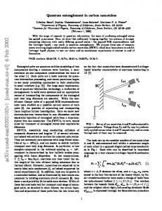
As shown in Fig. 2, the entanglement of formation EF (ρ) is a monotonically increasing function of the fidelity F for isotropic states in any dimension d. Therefore, by optimizing our QCM in terms of fidelity we maximize, at the same time, the entanglement of the clones measured by their entanglement of formation. The circles in Fig. 2 correspond to the maximal fidelity F that is achieved by our entanglement cloner, Eq. (12). They show as well the corresponding entanglement of formation in this dimension. The crosses mark the crossover between the expression of the fidelity corresponding to the second and third
0.8
0.6
0.4
0.2
0
0
0.1
0.2
0.3
0.4
0.5
0.6
0.7
0.8
0.9
F
FIG. 2: Entanglement of formation EF of the clone of a maximally-entangled input state versus the fidelity F of the clone for various dimensions d = 2 − 20 (the lowest curve corresponds to d = 2, while the highest curve corresponds to d = 20). The circles show the maximum achievable fidelity and the corresponding entanglement of formation. The crosses mark the crossover between the expression of the fidelity corresponding to the second and third lines of Eq. (22).
In order to visualize how the entanglement itself is cloned, we plot in Fig. 3 the entanglement of formation EF of the clones as a function of the entanglement of formation of the input ME state Ein , which is simply the von Neumann entropy of the reduced density matrix Ein = log2 d. We note that the entanglement of the clones is always less than one half the entanglement of the input state, while it asymptotically approaches this value for large d. The apparent “discontinuity” (if one can say so for a discrete graph) corresponds to d = 7, i.e., the crossover between the second and the third line of Eq. (22) when calculating the entropy of formation. In the limit of d → ∞, the third line of Eq. (22) tends to EF = F log2 d = F Ein . Since the cloner can be viewed, in this limit, as a classical random distribution process associated with a fidelity F = 1/2, then the entanglement of each clone tends to one half the entanglement of the initial state. In Fig. 3, we also plot the entanglement of formation resulting from the “local” cloner discussed above. Recall that this cloner differs from our optimal (non-local) entanglement cloner only by setting A = B. Therefore it is also covariant, satisfying Eq. (3), and all our arguments about the entanglement of formation of the clones are applicable to this cloner as well. Thus, using the fidelity of the clones (19), we may plot the entanglement of formation of the clones. We see that the local cloner
5 4
3.5
3
2.5
E
F2 1.5
1
0.5
0
0
1
2
3
4
E
5
6
7
8
in
FIG. 3: Entanglement of formation EF of the clones of a maximally-entangled state obtained by the optimal (nonlocal) cloner (◦) and the local cloner (+) versus the entanglement of the input state Ein for various dimensions d = 2−200. The apparent “discontinuity” in both curves is due to the crossover from the second to the third line of Eq. (22) for d ≥ 7 (optimal cloner) and d ≥ 13 (local cloner). Solid lines represent the asymptotics of EF for large d in both cases.
leads to a lower entanglement of formation, and even the asymptotics of EF for large d is no more than one fourth the entanglement of the input state. The reason is that in the limit of large d, the classical random distribution only succeeds with probability 1/2 independently for Alice’s and Bob’s components, so the fidelity is 1/4. Hence, EF → Ein /4. These observations confirm that by increasing the dimensionality, we make the system behavior look more and more classical. VI.
SEPARABILITY CONSERVATION
The last point to check is that our cloner does not create entanglement by itself, that is, it clones separable states into separable states. First, an important observation is that our cloner is such that the input-to-singleclone transformation is a PPT map. Using Eqs. (1) and (6), and tracing the joint state |SiR,a,b,A over the ancilla A and one of the clones, say b, we arrive at the following expression for the state of the reference and the other clone SR,a = |A|2 (11A ⊗ 11B )R,a
� + d2 (d2 + 2)|A|2 + 2|B|2 + 4d ℜ(A∗ B) ×(|φiA hφ|A ⊗ |φiB hφ|B )R,a � + d d|B|2 + 2 ℜ(A∗ B) ×(|φiA hφ|A ⊗ 11B + 11A ⊗ |φiB hφ|B )R,a (26)
where 11A is the identity operator in the joint space of Alice’s component of the reference R and clone a, while
Pd−1 |φiA = d−1/2 i=0 |iiA,R |iiA,a is a ME state in this same space. (The same notations are used for Bob’s analog quantities 11B and |φiB .) The cloning map is thus PPT since (SR,a )TB ≥ 0, where TB stands for the partial transposition with respect to Bob’s components of the reference R and clone a. This PPT property ensures that the cloning of any isotropic state cannot increase its fidelity, hence its entanglement of formation [11]. In particular, all separable isotropic states are necessarily transformed into separable clones. In order to generalize this separability conservation property to all separable input states, outside the restricted class of isotropic states, we consider the cloning of a product state ρA ⊗ ρB . By tracing (ρA ⊗ ρB )T SR,a over the reference R , we obtain for the first clone a state of the form ρa = |A|2 (11A ⊗ 11B )a � + (d2 + 2)|A|2 + 2|B|2 + 4d ℜ(A∗ B) (ρA ⊗ ρB )a � + d|B|2 + 2 ℜ(A∗ B) (ρA ⊗ 11B + 11A ⊗ ρB )a (27)
where 11A and 11B are identities in Alice’s and Bob’s subspaces of clone a, respectively. Since all terms in (27) are product states and all coefficients are positive semidefinite for all d, we verify that ρa is separable. By linearity of theP trace, this result also holds for P any linear comB bination i pi ρA i ⊗ρi with pi ≥ 0 and i pi = 1), that is for a generic separable state. Thus, we can conclude that our entanglement cloner transforms all initially separable states into separable clones. VII.
CONCLUSION
In conclusion, we have constructed an optimal (symmetric) entanglement cloner, which is universal over the set of d × d ME states in arbitrary dimension d. On one hand, all separable input states are cloned by this cloner into separable states. In addition, the entanglement of isotropic states cannot be increased by the cloner (and we conjecture this property holds in general for any input state). On the other hand, the entanglement of the clones of ME input states is maximum. The optimization of the parameters of our QCM was performed by maximizing the fidelity of the clones, but the monotonic behavior of the entanglement of formation as a function of the fidelity for isotropic states guarantees that such an optimization maximizes the entanglement of the clones at the same time. We expect that entanglement is cloned “monotonically” for all (including non-isotropic) states, that is, higher entangled states result in higher entangled clones, and therefore the ME input states are those which generate the clones with the maximum achievable entanglement. If this very natural assumption is right, then, based on our result, one can state that the maximal entanglement attainable by cloning is always below one half of the entanglement of the input state and saturates this value in the limit of large dimension d. This is consistent
6 with the idea that, since our QCM transforms separable states into separable clones, no additional entanglement is produced by cloning, so we can only split the entanglement of the input state between the two clones. This explains as well the asymptotic value of one fourth the initial entanglement for the local cloner at the limit of large d. It is natural to expect all these conclusions to be valid for asymmetric entanglement cloners as well.
port from the European Union under the projects RESQ (Grant No. IST-2001-37559) and SECOCQ (Grant No. IST-2002-506813), from the Communaut´e Fran¸caise de la Belgique under the “Action de Recherche Concert´ee” nr. 00/05-251, and from IAP program of Belgian federal government under Grant No. V-18.
Acknowledgments
We thank Louis-Philippe Lamoureux and Jaromir Fiurasek for helpful discussions. We acknowledge the sup-
[1] W.K. Wooters and W.H. Zurek, Nature (London) 299, 802 (1982); D. Dieks, Phys. Lett. 92A, 271 (1982). [2] V. Buˇzek and M. Hillery, Phys. Rev. A 54, 1844 (1996). [3] L.-Ph. Lamoureux, P. Navez, J. Fiur´ aˇsek, and N. Cerf, Phys. Rev. A, 69, 040301(R) (2004). [4] M. Hamermesh, Group Theory and its Application to Physical Problems, (Dover, Toronto, 1989). [5] N. J. Cerf, J. Mod Opt., 47, 187 (2000). [6] P. Navez and N.Cerf, Phys. Rev. A 68, 032313 (2003). [7] C.H. Bennett, D.P. DiVincenzo, J.A. Smolin, and
W.K. Wootters, Phys.Rev. A 54, 3824 (1996). [8] K.G.H. Vollbrecht and R.F. Werner, Phys. Rev. A 64, 062307 (2001). [9] M. Horodecki and P. Horodecki, Phys.Rev. A59, 4206 (1999). [10] B.M. Terhal and K.G.H. Vollbrecht, Phys. Rev. Lett, 85, 2625 (2000). [11] E. M. Rains, IEEE Trans.Inf.Theory, 47, 2921 (2001).