In this paper we develop closed-form solutions for the self-calibration of a stereo rig from a single general or ground-plane motion. The basic assumption.
Closed-form solutions for the Euclidean calibration of a stereo rig G. Csurka, D. Demirdjian, A. Ruf, and R. Horaud INRIA Rh^one-Alpes, 655 Av. de l'Europe, 38330 Montbonnot Saint Martin, France
Abstract. In this paper we describe a method for estimating the in-
ternal parameters of the left and right cameras associated with a stereo image pair. The stereo pair has known epipolar geometry and therefore 3-D projective reconstruction of pairs of matched image points is available. The stereo pair is allowed to move and hence there is a collineation relating the two projective reconstructions computed before and after the motion. We show that this collineation has similar but di�erent parameterizations for general and ground-plane rigid motions and we make explicit the relationship between the internal camera parameters and such a collineation. We devise a practical method for recovering four camera parameters from a single general motion or three camera parameters from a single ground-plane motion. Numerous experiments with simulated, calibrated and natural data validate the calibration method.
1 Introduction Traditional stereo vision systems use a single image pair to provide projective, a�ne, or Euclidean reconstruction. It has been clear that redundancy o�ered by further image pairs can signi cantly increase the quality and stability of visual reconstructions. Nevertheless, if the visual task is to recover metric structure, there are problems because both the intrinsic parameters (of the left and right cameras) and extrinsic ones (relative position and orientation of the two cameras) can vary over time. This is particularly critical when an active stereo head is being used. It is therefore important to be able to re-calibrate the stereo rig over time and over a small number of motions without using any special purpose calibration device. A number of authors investigated the relationship between projective, a�ne, and metric spaces in conjunction with a single camera undergoing rigid motions [10,6,7,13,15]. In [14] it is shown that there are many critical situations for which metric structure cannot be recovered. When image pairs are available one may use additional constraints. A�ne structure can be recovered from either pure translations [12], pure rotations [2] or ground-plane motions [1] of a stereo rig. For general motions, a�ne structure can be estimated from the eigenvector of a 3-D collineation [17] and metric structure can be estimated from two general motions [3]. Furthermore, in [8] it is shown that a�ne structure is an intrinsic property of a rigid stereo rig and that it can be easily recovered by combining any number of general motions.
In this paper we develop closed-form solutions for the self-calibration of a stereo rig from a single general or ground-plane motion. The basic assumption is that the stereo rig has the same internal and external parameters before and after the motion. More precisely, let P1 and P2 be two projective reconstructions obtained with an uncalibrated stereo rig before and after a rigid motion. These two reconstructions, i.e., a set of 3-D points, are related by a 4�4 collineation H12 which is related to the rigid motion D12 by ([17,3]): ? D HPE H ' HPE 12
1
12
(1)
As it will be shown below, an immediate consequence of this similarity relationship is that H12 can be factorized as �J�?1 where J is a real Jordan canonical form. We prove that this factorization is not unique and we show how to parameterize all such factorizations and how to estimate them in practice. Furthermore, we show that there exists a relationship between the left (or right) camera parameters and all possible factorizations of H12 . More precisely, let K be the upper triangular matrix associated with the left camera such that K33 = 1. We will show that (i) in the case of a general motion the matrix KK> is parameterized by a pencil of conics and that (ii) for a groundplane motion KK> is parameterized by a linear combination of three conics. Therefore, one constraint onto the entries of K is su�cient to estimate four intrinsic parameters from a single motion and two constraints onto the entries of K are necessary for estimating three intrinsic parameters from a single planar motion. As a consequence, a camera with zero image skew can be calibrated from a general motion and a camera with zero image skew and known aspect ratio can in turn be calibrated from one ground-plane motion. The method described in this paper has several advantages over previous stereo calibration approaches. The rst advantage is that a�ne calibration is not necessary prior to metric calibration as it is done with strati ed approaches. This is particularly important for ground-plane motions for which a�ne structure has proved di�cult to obtain. The second advantage is that all the computations are based on linear algebra techniques such as singular value decomposition. The third advantage is that, while a single motion is su�cient to calibrate, several motions can be combined in conjunction with a standard outliers rejection method in order to estimate the calibration parameters more robustly.
1.1 Paper organization The remainder of the paper is organized as follows. Section 2 brie y recalls the camera model and makes explicit the structure of KK> for a camera with zero skew and for a camera with zero skew and known aspect ratio. Section 3 recalls the mathematical properties associated with equation (1). Section 4 describes the real Jordan factorization of matrix H12 , analyses this factorization from a geometrical point of view, shows how to parameterize all possible factorizations, and describes a method to compute these factorizations in practice. Section 5 shows how to perform Euclidean calibration from the real Jordan factorization
of H12 for general and ground-plane motions. Section 6 validates the method with simulated and real data and Section 7 discusses the method in the light of the experimental results obtained so far.
2 Camera model and the absolute conic
A pinhole camera projects a point M from the 3-D projective space onto a point m of the 2-D projective plane. This projection can be written as m ' PM , where P is a 3�4 homogeneous matrix of rank equal to 3 and the sign ' designates the projective equality { equality up to a scale factor. If we restrict the 3-D projective space to the Euclidean space, then it is well known that P can be written as: PE = K ? R t � = ? KR Kt � (2) where R and t describe the orientation and the position of the camera in the chosen Euclidean frame. If we consider the standard camera frame as the 3-D Euclidean frame (the origin is the center of projection, the xy-plane is parallel to the image plane and the?z-axis�points towards the visible scene), the projection matrix becomes1 PE = K 03 . The most general form for the matrix of intrinsic parameters K is:
0� r u 1 K = @ 0 k� v A 0
(3) 0 0 1 where � is the horizontal scale factor, k is the ratio between the vertical and horizontal scale factors, r is the image skew and u0 and v0 are the image coordinates of the center of projection. The relation between the matrix K and the image of the absolute conic is C ' K?>K?1 [4]. Let us make explicit the dual of this conic, i.e., A = C?>: 0 �2 + r2 + u2 rk� + u v u 1 0 0 0 0 A ' KK> = @ rk� + u0v0 k2�2 + v02 v0 A (4) u0 v0 1 This means that A is symmetric and if we want to x the scale factor (A is de ned up to a scale) such that A = KK>, we need that A33 = 1. Equation (3) describes a ve-parameter camera. It will be useful to consider camera models with a reduced set of intrinsic parameters, as follows: { four-parameter camera with r = 0 (image skew), which means that the image is a rectangle { a sensible assumption. In this case the dual conic becomes: 0 �2 + u 2 u v u 1 0 0 0 0 A ' KK> = @ u0v0 k2�2 + v02 v0 A (5) u0 v0 1 0
1
We denote by 0n the n-vector containing n zeros.
which provides an additional constraint on the entries of A, i.e. A12 ? A13 A23 = 0. { three-parameter camera with r = 0 and k (aspect ratio) having a known value; for instance the value of k can be obtained from the physical size of a pixel. Therefore there is an additional constraint on the entries of A:
k2 (A11 ? A212 ) ? (A223 ? A22 ) = 0
3 Rigid motion of a stereo rig A stereo rig is composed of two cameras xed together. Let P and P0 be the projection matrices of the left and right cameras. We? can choose without �. In this 2 I 0 case loss of? generality a projective basis B such that P = 3 3 P � 0 0 > 0 P = H1 + e a ; �e [11], where H1 is the in nite homography between the left and right images, e0 is the right epipole, a an arbitrary 3-vector ? and � � is an arbitrary scale factor. It was shown in [8] that the 4-vector a> � has a simple but important geometric interpretation, namely it is the plane of in nity associated with the stereo pair. However, this plane is not used throughout this paper. Given a stereo rig with two projection matrices P and P0 , it is possible to compute the 3-D projective coordinates of a point M in the basis BP from the equations m ' PM and m0 ' P0 M , where m and m0 are the projections of M onto the left and right images. If we restrict the projective space to the Euclidean space and choose as basis BE the standard camera frame associated with the rst camera, P and P0 are given by:
? � ? � and P0E = K0R K0t PE = K 0 where K and K0 are the matrices of left and right intrinsic camera parameters, R and t describe the orientation and position of the right camera frame with respect to the left camera frame. The equations m ' PE M E and m0 ' P0E M E allow the estimation of M E { the 3-D Euclidean coordinates of a 3-D point in the basis BE . It is straightforward to show that, if HPE represents the collineation between the projective basis BP and the Euclidean frame BE , i.e., M E ' HPE M , we 3
have the followings relations:
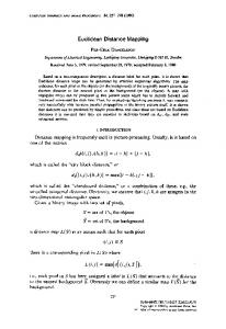
P ' PE HPE and P0 ' P0E HPE Indeed, from PM ' m ' PE M E ' PE HPE M it results that P ' PE HPE . The basic assumption throughout the paper is that the stereo rig performs a series of rigid motions and that during these motions K,K0 , R, and t remain constant, as shown in Figure 1. As the bases BP and BE are related to the 2 We denote by In the n � n matrix of identity.
H 12
BP
BP
N
M HPE
HPE P’
P
P
P’
BE
BE
D12
Fig. 1. Rigid motion of a stereo rig. stereo rig we can again use them to compute N and N E , the projective and Euclidean representations of the same physical point after the motion. Clearly, the relationship between the projective and Euclidean representations before the motion holds after the motion, N E ' HPE N . Let D12 be the 4�4 matrix describing the rigid motion performed by the stereo rig. We have N E = D12 M E and by substituting M E and N E with HPE M and HPE N we obtain:
N ' H?PE D HPE M 1
12
Consequently, the collineation between the two projective reconstructions (before and after the motion) (M and N ) is related to the rigid motion by the following formula:
H ' H?PE D HPE 12
1
12
(6)
In order to get rid of the scale p factor one may normalize H12 by dividing each term with sign(trace(H12)) 4 det(H12 ). With this normalization \'" becomes \=" and the eigenvalues of H12 and of D12 are the same. In what follows we assume that H12 has been normalized. The following proposition proved in [8] makes explicit the structure of HPE under the choice of the bases BP and BE :
Proposition 1. The 4�4 collineation HPE allowing the conversion of a projective reconstruction (basis BP ) obtained with a stereo rig into an Euclidean reconstruction (basis BE ) has the following structure: � ? � HPE = K 0 (7) 1
3
a> �
where K is the matrix of intrinsic parameters of the left camera and the equation of the plane at in nity in the projective basis BP .
? a> � � is
4 Algebraic preliminaries In this section we make explicit some algebraic properties of the 4�4 collineation H12 which are direct consequences of equation (6). The displacement matrix D12 has the form:
�R t � D= > 12
(8)
12
0 1 3
where R12 is a 3�3 rotation matrix and t12 represents the translation. Therefore the eigenvalues of D12 are fei� ; e?i� ; 1; 1g. A key issue with our approach is the distinction between the algebraic multiplicity of an eigenvalue and its geometric multiplicity. We recall the following de nitions (see [16,9]):
De nition 2. Let � be an eigenvalue of a matrix. Its algebraic multiplicity is the number of times that it occurs as a root of the corresponding characteristic polynomial.
De nition 3. The geometric multiplicity of an eigenvalue � is the dimension of the eigenspace associated with the eigenvalue �.
In the case of a rigid displacement the algebraic multiplicity of the eigenvalue
� = 1 is, in general, equal to 2 (it is equal to 4 if � = 0). However its geometric
multiplicity depends on whether the rigid motion is a screw or not and is equal to: { 1 in the case of general displacement, i.e., there is a translation along the screw axis { 2 in the case of planar motion (there is no translation along the axis or rotation). Therefore there are distinct calibration solutions for these two types of motion. Given matrix H12 similar to D12 , its eigenvalues are fei� ; e?i� ; 1; 1g as well. From [9] we have the following proposition.
Proposition 4. Let be a matrix with its eigenvalues equal to fei� ; e?i� ; 1; 1g. Then there exists a non-singular matrix � such that: 0 cos(�) ? sin(�) 0 0 1 B sin(�) cos(�) 0 0 CC �? = �J �?
= �B (9) " @ 0 0 1 "A 1
0
0
1
01
where " = 1, if the geometric multiplicity of the double eigenvalue � = 1 is 1, J" = J1, and " = 0 if the geometric multiplicity of the double eigenvalue � = 1 is equal to 2, J" = J0 .
Furthermore, if = D is a displacement, � = � is of form:
�Q t � � = >� �
(10) 0 1 where Q� is an orthogonal matrix, i.e � is a rotation or a re ection followed 3
by a translation.
Since J" is the matrix associated with the real Jordan canonical form, the factorizations introduced in the proposition above are called real Jordan factorizations.
4.1 Non uniqueness of the real Jordan factorization The real Jordan factorization described above is not unique. This non unicity is of crucial importance for our calibration method and we are going to give some insights into this property.
Proposition 5. The real Jordan factorization of a matrix is not unique. Moreover, = �J" �? and = �0 J" �0? are real Jordan factorizations if and only if there exists a matrix M commuting with J" , i.e. MJ" = J" M, such that �0 = �M. Proof: For any M commuting with J" , we have = �J" MM? �? = �MJ"(�M)? . Conversely, if = �J" �? = �0 J" �0? , results that �? �0 J" = J" (�? �0 )? . Hence �? �0 = M commutes with J" . � By making explicit the matrix equality MJ" = J" M, it is easy to derive the structure of M: { if " = 1 (general motion), M = Mg has 4 degrees of freedom and can be 1
1
1
1
1
1
1
1
1
1
written as:
0 � ? 0 0 1 B � 0 0 CC Mg = B @0 0 !A 0 0 0
(11)
{ if " = 0 (planar motion), M = Mp has 6 degrees of freedom and the form:
0 � ? 0 0 1 B � 0 0 CC Mp = B @0 0 !A 0 0 ��
(12)
1
{ if is a displacement, i.e. = �J" �?1 , �M, must be of form (10). Using this constraint we obtain: 0 cos( ) sin( ) 0 0 1 �Q t � C B ? sin( ) cos( ) 0 0 z z C B (13) Md = @ 0 0 �1 ! A = 0>3 1 0 0 0 1
4.2 The real Jordan factorization of a collineation
The real Jordan factorization will be used to decompose matrix H12 which maps two projective reconstructions obtained with the stereo rig before and after the motion. It is therefore important to describe how to obtain one such a factorization. Proposition 6. Let fei� ; e?i� ; 1; 1g be the eigenvalues of H12 and let v1; v2 be the eigenvectors associated with ei� and e?i� . (i) If the eigenvalue � = 1 has geometric multiplicity equal to 1, let u3 be the eigenvector associated with this eigenvalue and we obtain the following real Jordan factorization: (14) H12 = ? u1 u2 u3 w � J1 ? u1 u2 u3 w �?1 = �g J1 �?g 1 where u1 = v1 + v2 , u2 = i(v1 ? v2 ) are two real vectors and vector w is de ned by3 � (H ? I )?1u � w = 12 3 3 (15)
w4 with w4 chosen such that det(u1 ; u2 ; u3 ; w) 6= 0. (ii) If the eigenvalue � = 1 has geometric multiplicity equal to 2 let the vectors fu3 ; u4 g be a basis of the associated eigenspace and in this case the following
real Jordan factorization is obtained: (16) H12 = ? u1 u2 u3 u4 � J0 ? u1 u2 u3 u4 �?1 = �pJ0�?p 1 Proof: We show (ii) rst. From H12v1 = (cos(�) + i sin(�))v 1 and H12v2 = (cos(�) ? i sin(�))v 2 , by simple addition and subtraction results: � H u = cos(�)u + sin(�)u 12 1 1 2 (17) H12u2 = ? sin(�)u1 + cos(�)u2 Furthermore H12 u3 = u3 , H12 u4 = u4 and writing together with (17), using matrix notation, gives: 0 cos(�) ? sin(�) 0 0 1 � B sin(�) cos(�) 0 0 CC � ? ? H12 u1 u2 u3 u4 = u1 u2 u3 u4 B @ 0 0 1 0A 0 0 01 3 We denoted by A the 3 � 3 upper left block of a 4 � 4 matrix A and by a the rst 3 components ot the 4 vector a.
which is equivalent to (16). Second we prove (i). By combining equation (17) with H12 u3 = u3 we obtain:
0 cos(�) ? sin(�) 0 1 � � ? ? H u u u = u u u @ sin(�) cos(�) 0 A 12
1
2
1
3
2
3
0
0
1
By inspecting equation (14), we notice that w must verify:
H w =u +w 12
3
(18)
The rank of H12 ? I4 is equal to 3. We can assume that det(H12 ? I3 ) 6= 0 and construct the vector given by equation (15). If det(H12 ? I3 ) = 0, we can consider an other 3 � 3 block of the matrix H12 and apply the same method.
� Consequently, one way to compute a real Jordan factorization of a 4�4 collineation H is to compute its eigenvalues and associated eigenvectors. In practice H is estimated from image measurements and therefore it is corrupted 12
12
by noise. This noise can considerably perturbate the eigenvalues and eigenvectors of H12 [16]. Therefore we devised a simple method for computing the column vectors of matrix � without computing explicitly the eigenvalues of H12 . The latter is estimated up to a scale factor but after normalization one may notice that the trace has a simple form tracep(H12 ) = 2 + 2 cos(�). Therefore, we have cos(�) = trace(2H)?2 and sin(�) = 1 ? cos(�)2 . Finally, from equation (17) we obtain: � H ? cos(�)I ? sin(�)I �� u � 12 4 4 1 sin(�)I4 H12 ? cos(�) u2 = 08 which yields a solution for u1 and u2 . The eigenspace corresponding to the eigenvalue 1 is given by (H12 ? I4 )u = 04. In the noise-less case the rank of H12 ? I4 is equal to 3. However, when the data are corrupted by noise det(H12 ? I4 ) 6= 0 and an approximate solution must be found. In practice the singular value decomposition of H12 ? I4 allows to compute the eigenspace associated with the unit eigenvalue. If there is one small singular value, the geometric multiplicity is one and u3 is the vector corresponding to this singular value. If there are two small singular values, the geometric multiplicity is 2 and the two associated vectors are u3 and u4 .
5 Euclidean calibration We come back now to the basic equation associated with the rigid motion of a stereo rig H12 = H?PE1 D12 HPE . Consider rst a real Jordan factorization of
D , i.e D = �J�? . We obtain all the factorization by multiplying � with Md, equation (13): D = �MdJ"(�Md)? Consider now a real Jordan factorization of H obtained as described in Section 4.2. Again we multiply by matrix M to obtain all possible factorizations of H , i.e. H = �MJ" (�M)? . Replacing D and H in H = H?PE D HPE , results: �MJ"(�M)? = H?PE �MdJ"(H?PE �Md)? We immediately obtain H?PE �Md = �M and, from equations (7), (10) and 12
1
12
1
12
12
12
1
12
12
12
1
12
12
1
1
1
1
1
(13), results:
� K 0 �� Q t �� Q t � � KQ Q � � z z � � � z � � ? � a> K � 0> 1 0> 1 = 1
3 1
3
3
Furthermore, by considering only the upper-left 3�3 block matrices in this equation one obtains KQ� Qz = (�M) and nally the orthogonality of matrices Q� and Qz leads to the following relationship: KK> = (KQ� Qz )(KQ� Qz )> = (�M) (�M)> (19)
5.1 General motion
For a general motion the structure of matrix M is given by equations (14) and (11) and we have: �g Mg = ? �u1 + u2 �u2 ? u1 u3 !u3 + w � The dual of the image of the absolute conic becomes in this case: KK> = (�g Mg )(�g Mg )> = (|�2 {z + 2})(u1 u>1 + u2 u>2 ) + |{z}
2 u3 u>3 (20)
� � > > where ui = (ui1 ; ui2 ; ui3 ) for each ui = (ui1 ; ui2 ; ui3 ; ui4 ) , i = 1; 2; 3. Note that KK> depends merely on vectors u1 ; u2 ; u3 which have already
been estimated and on two further positive parameters � � 0 and � � 0. Therefore, in order to estimate A = KK> from a single movement two additional constraints are needed. As it was shown in Section 2, a four-parameter camera has exactly two constraints associated with the entries of A, namely: �A = 1 33 (21) A12 ? A13 A23 = 0 By combining (20) with (21) obtain the following solutions for � and �: Q2 (uj u3 ? u3uj ) � = ? Q2 3 j 3j=1 j 1 3 2 j1 2 3 2 3 j=1 (u3 (u1 u1 + u2 u2 ) ? u3 ((u1 ) + (u2 )2 )) 3 2 � = (u13?)2 �+(u(u3 )3 )2 (22) 1 2
where uji is the jth component of ui . Notice that one must check the sign of � and � since they must be, strictly positives by de nition. Once � and � are computed, one may determine KK> and compute the intrinsic parameters either directly from equation (5) or by Cholesky factorization.
5.2 Planar motion We consider now the case of a planar motion. In this case the structure of matrix M is de ned by equation (12) and the structure of matrix � is given by equation (16), i.e., matrices Mp and �p . Hence:
�pMp = ? �u + u �u ? u u + �u !u + �u � 1
2
2
1
3
4
3
4
and we obtain for the dual of the image of the absolute conic:
KK> = (�p Mp)(�pMp)> = (|� {z + })(u u> + u u> ) 2
2
1
�
+ |{z}
2 �
2
1
(23)
2
� � > � u u + ( ) (u u> + u u>) + ( � ) u u> |{z} |{z} 2
3
3
3
4
�
4
3
2
4
4
�2
In this case, A = KK> is de ned by vectors u1 ; u2 ; u3 ; u4 and by three undetermined parameters �; � and �. Since we have three unknown parameters, we need 3 constraints on A in order to calibrate the camera with a single motion. A three-parameter camera has the following three constraints associated with it (see Section 2):
8A = 1 < : Ak (A? A? AA ) =? 0(A ? A 33
12 2
13
11
23 2 12
2 23
22
)=0
(24)
By combining (23) with (24) we obtain the following formulae for � > 0, � > 0 and � 6= 0: 2 1 3 1 m ? u13 m3 ) + n2 (u33 m2 ? u23 m3 ) � = ? kk2 nn1 ((uu33 m 1 ? u1 m3 ) + n2 (u3 m2 ? u2 m3 ) 4
4
4
4
!
k2 m3 n1 u14 + m3 n2 u24 ? u34 (m1 n1 k2 + m2 n2 ) � = km3 (u1 (u3 m 1 ? u1 m3 ) ? u2 (u3 m2 ? u2 m3 ) + u3 (u2 m1 ? u1 m2 )) 3 4 4 3 4 4 3 4 4 3 3 2 1 ? � ( u + � u ) 3 4 �= (25) m3 with j 2 f1; 2; 3g, mj = uj1 u31 + uj2 u32 and nj = uj1 u32 ? u31 uj2 . Once � , � and � are thus computed and if the constraint � > 0 is veri ed, one 2
can determine the three camera parameters either in closed-form or by Cholesky factorization.
6 Experimental results In a rst series of experiments, the above developed methods are evaluated on synthetic image data in order to quantitatively study the accuracy of calibration as a function of image noise, and the type of movements considered. A second experiment compares the results of self-calibration and standard o�-line calibration on images of a particular calibration grid. The third experiment is to validate the use of our method for self-calibration of a stereo rig in an unknown real-word scene.
6.1 Synthetic data Synthetic stereo images showing a scene of about 40 3-D points are generated for ve di�erent points of view. The internal parameters of the two cameras were kept xed, such that projective reconstruction using [5] with the same projection matrices results in a representation of the scene in one and the same projective frame related to the stereo rig. The di�erent viewpoints are related by rigid motions of the rig and the conjugate collineations Hii+1 from position i to i +1 of projective space are estimated by the linear method presented in [8]. General screw motions and restricted planar motions are considered as camera motions, in order to comparatively study the performance of the respective methods of self-calibration. The in uence of image noise is evaluated by adding arti cial Gaussian noise with standard deviation varying from 0.3 to 2 pixels. In order to obtain signi cant results, closed-form self-calibration is performed for each single movement in the sequence and the average value of each parameter over the sequence is considered. For each parameter we compute the relative error between the estimated values ��u ; k�; u�0 ; v0� and the true values �u ; k; u0; v0 : �
�� = j �ju �? �j u j ; u
� �k = j kj?k kj j ;
�
�u = j uj0 u? uj 0 j 0
and
�
�v = j v0j v? vj 0 j 0
and for the principal point additionally the relative Euclidean distance between the points (u�0 ; v0� ) and (u0 ; v0 ) is considered:
s
� 2 + (v0 ? v0� )2 �u;v = (u0 ? u0u)2 + v2 0
0
The median of the relative errors over 100 trial runs is depicted in Figure 2 which demonstrates that accuracy of self-calibration degrades monotonically nicely with increasing measurement noise. Furthermore, calibration in the case of planar motion compares favorably with the case of general motion, given that a priori estimates of the xed parameters (skew and aspect ratio) are in the vicinity of the true values. Obviously, the estimates of the principal point (u0 ; v0 ) are less stable than those of the scale factors (�u ; k). On the one hand, the instability of the principal
Mean of four general motions
Mean of four planar motions
0.35
0.45
αu k u 0 v 0 (u0,v0)
0.3
α u u 0 v 0 (u ,v )
0.4
0
0.35
0
relative error over 100 trials
relative error over 100 trials
0.25
0.2
0.15
0.3
0.25
0.2
0.15
0.1 0.1 0.05 0.05
0
0
0.2
0.4
0.6
0.8
1 noise level
1.2
1.4
1.6
1.8
0
2
0
0.2
0.4
0.6
0.8
1 noise level
1.2
1.4
1.6
1.8
2
Fig. 2. Relative error in estimates of the intrinsic parameter from four general displacements (left) and four planar motions (right) at di�erent noise levels. Mean of n general motions
Mean of n planar motions
0.4
0.4
αu k u 0 v 0 (u0,v0)
0.35
0
0.25
0.2
0.15
0.1
0.25
0.2
0.15
0.1
0.05
0
0
0.3
relative error over 100 trials
relative error over 100 trials
0.3
α u u 0 v 0 (u ,v )
0.35
0.05
1
2
3
4 number of motions
5
6
7
0
1
2
3
4 number of motions
5
6
7
Fig. 3. The relative error in intrinsic parameters using an increasing number of motions. point is an intrinsic problem of camera calibration from noisy image measurements and was observed with most of the existing algorithms. On the other hand, an inaccurate principal point barely a�ects Euclidean reconstruction, as outlined in [8]. To quantify the possible gain in accuracy from combining several motions, closed-form self-calibration is performed over one to seven movements out of trajectories consisting of either a general motion or a planar motion. From 100 trial at a noise level of 1 pixel, the rst i movements of the trajectory were taken to calibrate and estimate the parameters by their average values. Figure 3 shows the evolution of the relative errors as a function of the number of motions which are considered. Obviously, using several motions instead of a of a single motion does not improve the accuracy associated with the estimation of �u and barely improves the accuracy associated with u0 ; v0 or k.
Method O�-line calibration General motion Planar motion
�
left camera
k u0 v0
right camera
�
k u0 v0
1534 .996 270 265 1520 .996 264 271 1550 .988 278 300 1533 .988 256 277 1570 k? 261 291 1561 k? 291 296
Table 1. Results for the left and right camera parameters using o�-line calibration and self-calibration. The results shown are means of several motions. We used k? = :996 as known value for planar motions.
6.2 Self-calibration with image pairs of a calibration grid
To justify the applicability of our method for camera self-calibration and to compare its e�ectiveness with that of standard o�-line methods, calibration is executed on images of a 3-D calibration grid. It consists of 100 circular target points, that are evenly distributed on three planes. Their 3-D positions are known with an accuracy of 0.02 mm, and their image projection are detected and localized at an accuracy of 0.05 pixel. The results of o�-line calibration using [4] and the results of applying our self-calibration methods to eight stereo image pairs of the grid are compared in Table 1, for the left and right cameras, respectively. Even-though no knowledge about 3D scene structure is required, self-calibration performs, for both types of motions, as well as o�-line calibration.
6.3 On-line self-calibration from image pairs of a 3-D scene
In order to validate the applicability of our method for camera self-calibration during runtime of a vision-system, i.e. for on-line calibration, we gathered 45 stereo images of a real-world scene from viewpoints which di�er merely by small motions of the stereo pair. To obtain point correspondences we used the following stereo tracking algorithm. Interest points are extracted from the rst pair and matched between the left and right images. Next, the points in the left image are tracked, as the stereo rig moves, over the sequence of images associated with the left camera motion. To obtain point matches associated with the image pair after the motion, the tracking is guided by the epipolar geometry. This algorithm makes use of the fact that the epipolar geometry remains unchanged during the motion of the stereo rig. Figure 4 shows the matches obtained with two image pairs. In contrast to the previous experiments, the matched points are no longer evenly distributed, neither in the image, nor in space. Even worse, mismatches may be present in the data. Additionally, interest points are no longer extracted with 0.05 pixel accuracy. Nevertheless, the camera parameters resulting from self-calibration are within the expected range and the behaviour of the method is consistent with the results obtained for synthetic data. Figure 5 depicts the distribution of parameter estimates obtained by closed-form calibration for about 1000 planar or general motions. Table 2 shows the average values of each parameter set.
Fig. 4. Two image pairs and their matched points.
7 Conclusion We proposed a method for self-calibration of a stereo rig from a single general or ground-plane motion. The basic assumption is that the stereo rig has the same internal and external parameters before and after the motion. In this case the collineation relating the two projective reconstructions performed at each position is conjugated to a displacement. By making explicit the algebraic properties of such a collineation, we derived a closed-form solution to recover four camera parameters from a single general motion or three camera parameters from a single ground-plane motion. One of the advantages of this approach is that calibration was done without explicitly computing a�ne structure. The second advantage is that all the computations are based on linear algebra techniques such as singular value decomposition, and hence it is easy to implement and has low computation cost. Therefore, it can be included in on-line perception-action cycle, such as visual servoing. One remarkable feature of our method is that it performs as well with small motions as with large ones. This has a crucial practical importance because it is much easier to nd matches between images that di�er by a small motion
Method O�-line calibration General motion Planar motion
�
left camera
right camera
k u0 v0
�
k u0 v0
1534 .996 270 265 1520 .996 264 271 1531 1.01 255 323 1508 1.05 211 334 1462 k? 154 246 1464 k? 143 259
Table 2. Results for the left and right camera parameters using o�-line calibration and self-calibration. The results shown are means of several motions. We used k? = :996 as known value for planar motions. Left camera
Left camera
Left camera
0.2
0.2
0.2
0.18
0.18
0.18
0.16
0.16
0.16
0.14
0.14
0.14
0.12
0.12
0.12
0.1
0.1
0.1
0.08
0.08
0.08
0.06
0.06
0.06
0.04
0.04
0.04
0.02
0.02
0
0
500
1000
1500 α
2000
2500
3000
0 −600
0.02
−400
−200
0
200
400
600
800
1000
1200
0 −500
0
Right camera
0.2
0.18
0.18
0.18
0.16
0.16
0.16
0.14
0.14
0.14
0.12
0.12
0.12
0.1
0.1
0.1
0.08
0.08
0.08
0.06
0.06
0.06
0.04
0.04
0.04
0.02
0.02
500
1000
1500 α u
2000
2500
3000
0 −600
1000
1500
1000
1500
Right camera
0.2
0
500 v 0
Right camera
0.2
0
0
u
u
0.02
−400
−200
0
200
400 u 0
600
800
1000
1200
1400
0 −500
0
500 v 0
Fig. 5. The distributions of the estimated intrinsic parameters. than for images that are far apart. One inconvenience is, however, that small motions may sometimes give rise to bad results simply because a rotation matrix which is closed to the identity matrix does not have the algebraic properties that are expected by the method. Nevertheless, these \bad" motions can be easily eliminated by simply checking the conditioning of the collineation H12 . Another source of errors is the sensitivity of the method to the accuracy with which the interest points are located and matched as well as the 3-D distribution of these points. This problem has been observed with both synthetic and real data. Interesting enough, the matrix conditioning analysis outlined above works well to eliminate such badly distributed data. In the future we plan to investigate more thoroughly the relationship between bad calibration and the numerical conditioning of the problem and to combine closed-form calibration methods with statistically robust methods.
References 1. P. A. Beardsley and A. Zisserman. A�ne calibration of mobile vehicles. In Proceedings of Europe-China Workshop on Geometrical Modelling and Invariants for Computer Vision, pages 214{221, Xi'an, China, April 1995. Xidan University Press. 2. P.A. Beardsley, I.D. Reid, A. Zisserman, and D.W. Murray. Active visual navigation using non-metric structure. In E. Grimson, editor, Proceedings of the 5th International Conference on Computer Vision, Cambridge, Massachusetts, USA, pages 58{64. ieee Computer Society Press, June 1995. 3. F. Devernay and O. Faugeras. From projective to Euclidean reconstruction. In Proceedings Computer Vision and Pattern Recognition Conference, pages 264{269, San Francisco, CA., June 1996. 4. O. D. Faugeras. Three Dimensional Computer Vision: A Geometric Viewpoint. MIT Press, Boston, 1993. 5. R. Hartley and P. Sturm. Triangulation. Computer Vision and Image Understanding, 68(2):146{157, 1997. 6. R. I. Hartley. Euclidean reconstruction from uncalibrated views. In Mundy Zisserman Forsyth, editor, Applications of Invariance in Computer Vision, pages 237{ 256. Springer Verlag, Berlin Heidelberg, 1994. 7. A. Heyden and K. � Astrom. Euclidean reconstruction from constant intrinsic parameters. In Proceedings of the 13th International Conference on Pattern Recognition, Vienna, Austria, volume I, pages 339{343, August 1996. 8. R. Horaud and G. Csurka. Self-calibration and euclidean reconstruction using motions of a stereo rig. In Proceedings of the 6th International Conference on Computer Vision, Bombay, India, pages 96{103, January 1998. 9. R.A. Horn and C.R. Johnson. Matrix analysis. Cambridge University Press, 1985. 10. Q-T. Luong and O. D. Faugeras. Self-calibration of a moving camera from point correspondences and fundamental matrices. International Journal of Computer Vision, 22(3):261{289, 1997. 11. Q.T. Luong and T. Vieville. Canonic representations for the geometries of multiple projective views. In Proceedings of the 3rd European Conference on Computer Vision, Stockholm, Sweden, pages 589{599, May 1994. 12. T. Moons, L. Van Gool, M. Proesmans, and E Pauwels. A�ne reconstruction from perspective image pairs with a relative object-camera translation in between. IEEE Transactions on Pattern Analysis and Machine Intelligence, 18(1):77{83, January 1996. 13. M. Pollefeys and L. Van Gool. A strati ed approach to metric self-calibration. In Proceedings of the Conference on Computer Vision and Pattern Recognition, Puerto Rico, USA, pages 407{412. ieee Computer Society Press, June 1997. 14. P. Sturm. Critical motion sequences for monocular self-calibration and uncalibrated euclidean reconstruction. In Proceedings of IEEE Computer Society Conference on Computer Vision and Pattern Recognition, pages 1100{1105, Puerto-Rico, June 1997. 15. B. Triggs. Autocalibration and the absolute quadric. In Proceedings of the Conference on Computer Vision and Pattern Recognition, Puerto Rico, USA, pages 609{614. ieee Computer Society Press, June 1997. 16. J.H. Wilkinson. The algebraic eigenvalue problem. Clarendon Press - Oxford, 1965. 17. A. Zisserman, P. A. Beardsley, and I. D. Reid. Metric calibration of a stereo rig. In Proc. IEEE Workshop on Representation of Visual Scenes, pages 93{100, Cambridge, Mass., June 1995.