Hindawi Publishing Corporation Mathematical Problems in Engineering Volume 2013, Article ID 519432, 10 pages http://dx.doi.org/10.1155/2013/519432
Research Article Closed-Loop Identification Applied to a DC Servomechanism: Controller Gains Analysis Roger Miranda Colorado and Gamaliel Contreras Castro Universidad Polit´ecnica de Victoria, Avenida Nuevas Tecnolog´ıas 5902, Parque Cient´ıfico y Tecnol´ogico de Tamaulipas, 87138 Ciudad Victoria, TAMPS, Mexico Correspondence should be addressed to Roger Miranda Colorado;
[email protected] Received 13 June 2013; Accepted 11 October 2013 Academic Editor: Wudhichai Assawinchaichote Copyright © 2013 R. Miranda Colorado and G. Contreras Castro. This is an open access article distributed under the Creative Commons Attribution License, which permits unrestricted use, distribution, and reproduction in any medium, provided the original work is properly cited. Usually, when parameter identification is applied, there are some gains related to the identification algorithm whose value must be carefully adjusted in order to obtain a good performance of the algorithm. However, when performing closed loop identification, there are some other constants that in general are not taken into account for the identification algorithm: the controller gains, which may appear inside the identification algorithm, specifically in the regressor vector, which is very important for the parameter convergence according to the persistence of excitation condition. Therefore, the effect of these gains on the estimated parameters should be analyzed so that better estimates can be obtained. This paper addresses the behavior of the parameter estimates for a closed-loop identification methodology applied to a DC servomechanism with a bounded perturbation signal and a PD controller. It is shown that, with this perturbation, the parameter estimates converge to a region whose size can be modified not only by varying the identification algorithm gains but also by modifying the P and D controller gains in a suitable way.
1. Introduction It is well known that servomechanisms are fundamental in modern robotic and mechatronic systems for industrial applications where high speed and high precision are of prime importance. On the other hand, in order to apply model-based tuning methods it is necessary to apply an identification algorithm to the servomechanism and, if it is required, to design a high performance controller where a small steady state tracking error and high precision are necessary. Besides, the system parameters are also important to know if the system itself behaves as it should, for example, by evaluating its performance with some specified test signals. Thus, parameter identification plays a very important role for designing a controller as pointed out from several points of view [1–4]. For a DC servomechanism, there are several techniques that may be applied for identifying its parameters, when the servomechanism operates in open loop and in closed loop. However, it is important to note that if the variable of interest is the servo position, then a linear model of
a servomechanism contains a pole on the imaginary axis, thus making the system not BIBO stable, that is, a bounded input applied to the servomechanism would not produce a bounded position and this may lead to undesired effects, for example, in robotic applications. Therefore, for security reasons, parameter identification should be performed in closed loop. One way to characterize the system identification algorithms is [5, 6] (i) direct methods and (ii) indirect methods. Many of the identification procedures using a linear controller [7–9] fall into the category of direct methods; that is, the parameter identification procedures are applied without regard to the controller being used to close the loop. On the other hand, if a technique takes into account the controller structure, then it falls into the category of indirect methods. As mentioned before, for security reason it is better to estimate the system parameters with the system working in closed loop. One way to perform closed loop parameter identification of a servomechanism is with the relay-based techniques [10–12], which are widespread for servo identification. The idea with this methodology is to close the loop
2 through a relay in order to obtain a sustained oscillation and then the values of the frequency and amplitude allows identifying a model of the system. The relay based techniques may work well; however, the reference signal used for exciting the system becomes constant in many time instants, and then no control is being applied in that time and then the effect of the disturbances may affect the estimates obtained with this methodology. Besides, tuning of the relay controller can be cumbersome and no one of the reviewed methods takes explicitly into account the disturbances affecting the servomechanism. References [7–9, 13–15] propose methods for closed loop identification of position-controlled servos where the loop is closed using a linear controller. The approach proposed in [13, 14] uses a PD controller to close the loop and an on-line gradient algorithm allows estimating a linear and nonlinear model of a servomechanism. Also, in [15] a twostep identification method for estimating the four parameters of a nonlinear model of a position control servomechanism is presented, where the proposed identification scheme relies on the theory of operational calculus. However, the effect of perturbations is considered only for constant values. On the other hand, a common technique used for identifying DC servomechanisms is based on the least squares algorithm. In [16], an approach for identifying a DC motor is presented considering the Coulomb friction and dead zone using a recursive discrete time least squares algorithm with forgetting factor using a Hammerstein model for the motor. In [17], second-order sliding modes approach is applied for estimating the parameters of a DC motor operating in open-loop and closed loop, while in [18] the inertia of a second-order model of a DC servomechanism driving a human assistive system is identified using Bode plots obtained from input-output measurements. Finally, another interesting approach is presented in [2, 4], where an online algebraic identification method is proposed. Besides, [19, 20] show how this methodology can be used for parameter identification of a DC motor and also this methodology was used and modified in [21] introducing a batch least squares algorithm for estimating the parameters of an induction motor. All the previous works consider in general the importance of some gains related with the identification algorithm for closed-loop identification. However, in some cases (as that presented in [13, 14]) the controller gains get involved in with some important elements for the identification scheme, for example, in the regressor vector. In this case, it has not been analyzed which effect actually has such gains in the parameter identification procedure and how the parameter estimates will behave when a disturbance is affecting the system. Then, this work presents the analysis of a closed loop identification algorithm for a perturbed position-controlled DC servomechanism where a PD controller closes the loop and achieves stability without knowledge about the servomechanism parameters. Theoretical results show that, when the perturbation signal is identically zero, exponential convergence can be claimed, and in the presence of a bounded perturbation it is possible to obtain a region Ω𝛿 where the parameter estimates belong. What’s more, it will be shown that this region can be made arbitrarily small if
Mathematical Problems in Engineering the controller gains are tuned properly. Some simulations depict the behavior of the region Ω𝛿 , showing the effect that the controller gains have on the estimated parameters. The paper is organized as follows. Section 2 is devoted to present preliminary theoretical results of passivity based control, adaptive control, and the general description of the DC servomechanism. Section 3 presents the analysis for closed loop identification of the servomechanism when no disturbances are affecting the system and the exponential stability of the overall identification scheme is shown. Section 4 extends the analysis for the perturbed case and Section 5 deals with the analysis of the results. Finally, Section 6 gives some concluding remarks.
2. Preliminary Results The closed loop identification analysis that will be presented is based on some results related with passivity theory and adaptive control, and thus the following results are worth presenting. 2.1. Passivity and Adaptive Control. As pointed out before, the aim of this work is to show the convergence properties of the identification algorithm with respect to the value of the controller gains. To this end it will be necessary to use the observability property given in [22] and some results of passivity and stability that will be described in the following. Let us consider the linear time-varying system [𝐶(𝑡), 𝐴(𝑡)] defined by 𝑥̇ = 𝐴 (𝑡) 𝑥 (𝑡) , 𝑦 (𝑡) = 𝐶 (𝑡) 𝑥 (𝑡) ,
(1)
where 𝑥(𝑡) ∈ 𝑅𝑛 , 𝑦(𝑡) ∈ 𝑅𝑚 , while 𝐴(𝑡) ∈ 𝑅𝑛×𝑛 and 𝐶(𝑡) ∈ 𝑅𝑚×𝑛 are piecewise continuous functions. A system [𝐶(𝑡), 𝐴(𝑡)] is said to be uniformly completely observable (UCO) [22] if there exist strictly positive constants {𝛽1 , 𝛽2 , 𝛿} such that, for all 𝑡0 ≥ 0, 𝛽1 𝐼 ≤ 𝑁(𝑡0 , 𝑡0 + 𝛿) ≤ 𝛽2 𝐼, where 𝑁(𝑡0 , 𝑡0 + 𝛿) ∈ 𝑅𝑛×𝑛 is the so-called observability Gramian as 𝑁 (𝑡0 , 𝑡0 + 𝛿) = ∫
𝑡0 +𝛿
𝑡0
Φ𝑇 (𝜏, 𝑡0 ) 𝐶𝑇 (𝜏) 𝐶 (𝜏) Φ (𝜏, 𝑡0 ) 𝑑𝜏, (2)
where Φ(𝜏, 𝑡0 ) is the state transition matrix associated with 𝐴(𝑡). Now, assume that, for all 𝛿 > 0, there exists 𝑘𝛿 > 0 such 𝑡 +𝛿 that, for all 𝑡0 ≥ 0, ∫𝑡 0 ‖𝐾(𝜏)‖2 𝑑𝜏 ≤ 𝑘𝛿 , where the matrix 𝐾 0 corresponds to the system under output injection as 𝑤̇ = {𝐴 (𝑡) + 𝐾 (𝑡) 𝐶 (𝑡)} 𝑤 (𝑡) , 𝑧 (𝑡) = 𝐶 (𝑡) 𝑤 (𝑡) ,
(3)
with 𝑤(𝑡) ∈ 𝑅𝑛 , 𝐾(𝑡) ∈ 𝑅𝑛×𝑚 , and 𝑧(𝑡) ∈ 𝑅𝑚 . Then, the system [𝐶, 𝐴] is UCO if and only if [𝐶, 𝐴 + 𝐾𝐶] is UCO, where the term 𝐾𝐶 stands for the output injection term as indicated in [22]. Moreover, if the observability Gramian of the system [𝐶, 𝐴] satisfies the previous upper and lower bounds on 𝑁,
Mathematical Problems in Engineering
3
then the observability Gramian of the system [𝐶, 𝐴 + 𝐾𝐶] satisfies these inequalities with identical 𝛿 and 𝛽1 =
𝛽1 (1 + √𝑘𝛿 𝛽2 )
𝛽2 = 𝛽2 exp (𝑘𝛿 𝛽2 ) .
,
(4)
Now assume that 𝑓(𝑡, 𝑥) : 𝑅+ × 𝑅𝑛 → 𝑅𝑛 has continuous and bounded first partial derivatives in 𝑥(𝑡) and is piecewise continuous in 𝑡 for all 𝑥 ∈ 𝐵ℎ , 𝑡 ≥ 0. Then, the following statements are equivalent [22]. (1) 𝑥 = 0 is an exponentially stable equilibrium point of 𝑥̇ = 𝑓(𝑡, 𝑥), 𝑥(𝑡0 ) = 𝑥0 . (2) There exists a function 𝑉(𝑡, 𝑥) and some strictly positive constants ℎ , 𝛼1 , 𝛼2 , 𝛼3 , and 𝛼4 such that, for all 𝑥 ∈ 𝐵ℎ and 𝑡 ≥ 0, 𝛼1 ‖𝑥‖2 ≤ 𝑉(𝑡, 𝑥) ≤ 𝛼2 ‖𝑥‖2 , ̇ 𝑥)|𝑥=𝑓(𝑡,𝑥) ≤ −𝛼3 ‖𝑥‖2 , and |𝜕𝑉(𝑡, 𝑥)/𝜕𝑥| ≤ 𝛼4 ‖𝑥‖. 𝑉(𝑡, ̇ Now, if there exists a function 𝑉(𝑡, 𝑥) and strictly positive constants 𝛼1 , 𝛼2 , 𝛼3 , and 𝛿, such that, for all 𝑥 ∈ 𝐵ℎ , ̇ 𝑥)|𝑥=𝑓(𝑡,𝑥) ≤ 𝑡 ≥ 0: 𝛼1 ‖𝑥‖2 ≤ 𝑉(𝑡, 𝑥) ≤ 𝛼2 ‖𝑥‖2 , 𝑉(𝑡, ̇ 𝑡+𝛿
0 and ∫𝑡 𝑑𝑉(𝜏, 𝑥(𝜏))/𝑑𝜏|𝑥=𝑓(𝑡,𝑥) 𝑑𝜏 ≤ −𝛼3 ‖𝑥‖2 then, 𝑥(𝑡) ̇ converges exponentially to zero. Finally [23], the state equation [𝐴, 𝐵, 𝐶, 𝐷] is a minimal ̂ if and only if realization of a proper rational function 𝑔(𝑠) (𝐴, 𝐵) is controllable, (𝐴, 𝐶) is observable, or if and only ̂ ̂ if dim(𝐴) = deg(𝑔(𝑠)), where 𝑔(𝑠) = 𝑁(𝑠)/𝐷(𝑠) and ̂ deg(𝑔(𝑠)) = deg(𝐷(𝑠)). In the next definitions, let us consider the system Π defined as 𝑥̇ (𝑡) = 𝑓 (𝑥, 𝑢) , { { Π : {𝑥 (0) = 𝑥0 ∈ 𝑅𝑛 , { {𝑦 (𝑡) = 𝐻 (𝑥, 𝑢) ,
(5)
where 𝑥 ∈ 𝑅𝑛 is the state vector, 𝑢 ∈ 𝑅𝑚 the input, and 𝑦 ∈ 𝑅𝑚 the system output. Consider the set Ξ of 𝑛 dimensional real valued functions 𝑓(𝑡) : 𝑅+ → 𝑅𝑛 and define the set ∞ 𝐿 2 = {𝑥 ∈ Ξ : ‖𝑓‖22 = ∫0 ‖𝑓(𝑡)‖2 𝑑𝑡 < ∞}, with ‖ ⋅ ‖2 the Euclidean norm. This set constitutes a normed vector space with the field 𝑅 and norm ‖ ⋅ ‖2 . Let us introduce the extended space 𝐿 2𝑒 as 𝑇
2 2 𝐿 2𝑒 = {𝑥 ∈ Ξ : 𝑓2𝑇 = ∫ 𝑓 (𝑡) 𝑑𝑡 < ∞, ∀𝑇} , 0
(6)
where 𝐿 2 ⊂ 𝐿 2𝑒 . In the same way, let us introduce the inner product and the truncated inner product of functions 𝑢 and 𝑦 as ∞
(𝑢, 𝑦) = ∫ 𝑢𝑇 (𝑡) 𝑦 (𝑡) 𝑑𝑡, 0
𝑇
(7) 𝑇
(𝑢, 𝑦)𝑇 = ∫ 𝑢 (𝑡) 𝑦 (𝑡) 𝑑𝑡. 0
The system (5) is dissipative [24] with respect to the supply rate 𝜔(𝑢, 𝑦) : 𝑅𝑚 × 𝑅𝑚 → 𝑅 if and only if there exists a
storage function: 𝑅𝑛 → 𝑅≥0 , such that 𝐻(𝑥(𝑇)) ≤ 𝐻(𝑥(0)) + 𝑇
∫0 𝜔(𝑢(𝑡), 𝑦(𝑡))𝑑𝑡, for all 𝑢(𝑡), all 𝑇 ≥ 0, and all 𝑥0 ∈ 𝑅𝑛 . The system is passive if its supply rate is given by (𝑢, 𝑦) = 𝑢𝑇 𝑦. It is input strictly passive (ISP) if there exists a positive constant 𝛿𝑖 such that the supply rate can be expressed as (𝑢, 𝑦) = 𝑢𝑇 𝑦 − 𝛿𝑖 ‖𝑢‖2 , 𝛿𝑖 > 0. Finally, it is output strictly passive (OSP) if there exists a positive constant 𝛿0 such that the supply rate can be expressed as (𝑢, 𝑦) = 𝑢𝑇 𝑦 − 𝛿𝑜 ‖𝑦‖2 , 𝛿𝑜 > 0. The system (5) is called 𝐿 2 finite gain stable if there exists a positive constant 𝛾 such that for any initial condition 𝑥0 there exists a finite constant 𝛽(𝑥0 )such that ‖𝑦‖2𝑇 ≤ 𝛾‖𝑢‖2𝑇 + 𝛽(𝑥0 ) and one important result from [24] is that if Π : 𝑢 → 𝑦 is OSP, then it is 𝐿 2 stable. ̇ A state space system 𝑥(𝑡) = 𝑓(𝑥), 𝑥 ∈ 𝑅𝑛 , is zero state observable from the output 𝑦(𝑡) = ℎ(𝑥) if, for all initial conditions 𝑥(0) ∈ 𝑅𝑛 , the output 𝑦(𝑡) ≡ 0 implies that 𝑥(𝑡) ≡ 0. It is zero state detectable if 𝑦(𝑡) ≡ 0 implies that lim𝑥(𝑡) = 0 as 𝑡 → ∞. Regarding the identification algorithms, the persistence excitation (PE) condition is very important and its definition is given now according to [22]: a vector 𝜙 : 𝑅+ → 𝑅2𝑛 is persistently exciting (PE) if there exist constants {𝛼1 , 𝛼2 , 𝛿} > 0 such that 𝛼1 𝐼 ≤ ∫
𝑡0 +𝛿
𝑡0
𝜙 (𝜏) 𝜙𝑇 (𝜏) 𝑑𝜏 ≤ 𝛼2 𝐼,
∀𝑡0 ≥ 0.
(8)
Besides, let 𝑤 : 𝑅+ → 𝑅2𝑛 . If 𝑤 is PE, the signals {𝑤, 𝑤}̇ belong to the space 𝐿 ∞ , and 𝑈 is a rational stable strictly proper minimum phase transfer function, then 𝑈(𝑤) is PE. Theorem 1 (small signal I/O stability, [22]). Consider the perturbed system 𝑥̇ = 𝑓(𝑡, 𝑥, 𝑢), 𝑥(0) = 𝑥0 and the unperturbed system 𝑥̇ = 𝑓(𝑡, 𝑥, 0), 𝑥(0) = 𝑥0 , where 𝑡 ≥ 0, 𝑥 ∈ 𝑅𝑛 , and 𝑢 ∈ 𝑅𝑚 . Let 𝑥 = 0 be an equilibrium point of the unperturbed system, that is, 𝑓(𝑡, 0, 0) = 0, for all 𝑡 ≥ 0. Let 𝑓 be piecewise continuous in 𝑡 and have continuous and bounded first partial derivatives in 𝑥 for all 𝑡 ≥ 0, 𝑥 ∈ 𝐵ℎ , 𝑢 ∈ 𝐵𝑐 . Let 𝑓 be Lipchitz in u, with Lipchitz constant 𝑙𝑢 , for all 𝑡 ≥ 0, 𝑥 ∈ 𝐵ℎ , 𝑢 ∈ 𝐵𝑐 . Let 𝑢 ∈ 𝐿 ∞ . If 𝑥 = 0 is an exponentially stable equilibrium point of the unperturbed system, then the perturbed system is small-signal 𝐿 ∞ stable; that is, there exist 𝛾∞ , 𝑐∞ > 0, such that ‖𝑢‖∞ < 𝑐∞ implies that ‖𝑥‖∞ ≤ 𝛾∞ ‖𝑢‖∞ < ℎ, where 𝑥 is the solution of 𝑓(𝑡, 𝑥, 𝑢) starting at 𝑥0 = 0. There exists 𝑚 ≥ 1 such that, for all ‖𝑥0 ‖ < ℎ/𝑚, 0 < ‖𝑢‖∞ < c∞ implies that 𝑥(𝑡) converges to a 𝐵𝛿 ball of radius 𝛿 = 𝛾∞ ‖𝑢‖∞ < ℎ; that is, for all 𝜑 > 0, there exists 𝑇 ≥ 0 such that ‖𝑥(𝑡)‖ ≤ (1 + 𝜑)𝛿 for all 𝑡 ≥ 𝑇, along the solutions of 𝑓(𝑡, 𝑥, 𝑢) starting at 𝑥0 . Also for 𝑡 ≥ 0, ‖𝑥(𝑡)‖ < ℎ. 2.2. Model of the DC Servomechanism. The closed loop identification analysis that will be presented considers the model of a perturbed DC servomechanism described by the following equation: 𝐽𝑞 ̈ + 𝑓𝑞 ̇ (𝑡) = 𝑘𝑢 (𝑡) + ]1 (𝑡) = 𝜏 (𝑡) + ]1 (𝑡) ,
(9)
where 𝐽, 𝑓, 𝑘, 𝑢, ]1 , and 𝜏(𝑡) = 𝑘𝑢(𝑡) are the inertia, viscous friction coefficient, amplifier gain, input voltage, perturbation
4
Mathematical Problems in Engineering
signal, and torque input, respectively. The perturbation signal may be due to possibly constant disturbances or parasitic voltages appearing inside the amplifier. The model (9) can be rewritten as 𝑞V̈ (𝑡) = −𝑎𝑞 ̇ (𝑡) + 𝑏𝑢 (𝑡) + ] (𝑡) ,
(10)
where 𝑎 = 𝑓/𝐽 and 𝑏 = 𝑘/𝐽 are positive constants and ̇ are the servo angular position and ] = ]1 /𝐽 and {𝑞(𝑡), 𝑞(𝑡)} velocity, respectively. It is also assumed that the perturbation signal is bounded, that is: ‖]1 (𝑡)‖ ≤ 𝛽, 𝛽 ∈ 𝑅+ . In the following it will be shown that there exists a region Ω𝛿 where the parameter estimates converge, even in the presence of the perturbation signal ](𝑡). Furthermore, it will be shown that the size of this region can be arbitrarily reduced by increasing the controller gains employed for stabilizing the servomechanism. This analysis will consider two cases. (i) Closed loop identification of the unperturbed DC servomechanism, where the main objective will be to get a formula to estimate the system parameters and show the condition under which the system is exponentially stable. (ii) Closed loop identification of the perturbed DC servomechanism where the existence of the region Ω𝛿 will be shown where the parameter estimates converge, when a perturbation signal affects the system.
3. Closed-Loop Identification Algorithm: Nonperturbed Case This section describes the closed loop identification approach and the way the parameter updating law is constructed. Besides, it is proved that under some assumptions the overall system is exponentially stable. Then, first the stability analysis will be presented to ensure the asymptotic stability of the closed loop system and the parameter error dynamics. Later, the system exponential stability property will be established. 3.1. Stability Analysis and Parameter Convergence. The closed loop identification analysis to be described is similar to that presented in [14] and depicted in Figure 1. For this (unperturbed) case, it will be considered that ](𝑡) is identically zero, leading to the following unperturbed servo model: 𝑞 ̈ (𝑡) = −𝑎𝑞 ̇ (𝑡) + 𝑏𝑢 (𝑡) .
(11)
The closed loop identification methodology consists of selecting a model of (11) with the following dynamics: 𝑎𝑞𝑒̇ (𝑡) + ̂𝑏𝑢𝑒 (𝑡) , 𝑞𝑒̈ (𝑡) = −̂
(12)
where 𝑞𝑒 (𝑡) is the estimated servo position, 𝑞𝑒̇ (𝑡) the estimated velocity, {̂ 𝑎, ̂𝑏} are the estimates of {𝑎, 𝑏}, and 𝑢𝑒 the control law for the estimated model. Then, the loop is closed around the real servomechanism and its model by using two PD controllers, where the same gains are used for both of them. Now let us define the output error 𝜀(𝑡) = 𝑞(𝑡) − 𝑞𝑒 (𝑡), and then this error and its time derivative are employed to
feed an identification algorithm which estimates the system parameters and updates them in the estimated model. All this procedure is now theoretically summarized. For closing the loop around the unperturbed system and its model, let us consider the PD controllers u(t) and 𝑢𝑒 (𝑡) as ̇ and 𝑢𝑒 (𝑡) = 𝑘𝑝 𝑒𝑒 (𝑡) − 𝑘𝑑 𝑞𝑒̇ (𝑡), follows: 𝑢(𝑡) = 𝑘𝑝 𝑒(𝑡) − 𝑘𝑑 𝑞(𝑡) where 𝑒(𝑡) = (𝑞𝑑 (𝑡) − 𝑞(𝑡)), 𝑒𝑒 (𝑡) = (𝑞𝑑 (𝑡) − 𝑞𝑒 (𝑡)), 𝑞𝑑 (𝑡) is the reference signal, and 𝑘𝑝 > 0, 𝑘𝑑 > 0 the proportional and derivative controller gains which are used in both controllers. Then, the system (11) in closed loop with 𝑢(𝑡) leads to the next closed-loop dynamics (for the sake of simplicity, from now on the time argument will be omitted) as Σ1 : 𝑞 ̈ = − (𝑎 + 𝑏𝑘𝑑 ) 𝑞 ̇ + 𝑏𝑘𝑝 𝑒,
(13)
while the system (12) in closed loop with 𝑢𝑒 (𝑡) leads to the following dynamics: 𝑎 + ̂𝑏𝑘𝑑 ) 𝑞𝑒̇ + ̂𝑏𝑘𝑝 𝑒𝑒 . Σ2 : 𝑞𝑒̈ = − (̂
(14)
By using the Routh-Hurwitz criterion, it is easy to show that the control law 𝑢(𝑡) stabilizes the unperturbed servo model (11). However, even when the system (13) is stable, the same conclusion cannot be drawn for (14), because the coefficients of this estimated model (i.e., 𝑎̂, ̂𝑏) are updated by one identification algorithm to be described later, and then these parameters are time varying; therefore, it is necessary to analyze the stability of (14). From the definition of 𝜀(𝑡), it is possible to evaluate its second time derivative and employing (13) and (14), the error dynamics is established as follows: .. 𝜀 +𝑐𝜀 ̇ + 𝑏𝑘𝑝 𝜀 = 𝜃̃ 𝑇 𝜙,
(15)
̃ is the parameter error vector, where 𝑐 = (𝑎 + 𝑏𝑘𝑑 ) > 0, 𝜃(𝑡) and 𝜙(𝑡) is the so-called regressor vector, where 𝜃̃ = 𝜃̂ − 𝜃 = (̂ 𝑎 − 𝑎, ̂𝑏 − 𝑏)𝑇 , 𝜙(𝑡) = (𝑞𝑒̇ , −𝑢𝑒 )𝑇 , with 𝜃̂ being the estimate of 𝜃. In order to analyze the behavior of the signals involved in the error dynamics (15), passivity based arguments will be used [24, 25]. To this end, let 𝑥 = (𝜀, 𝜀)̇ 𝑇 be the state vector of (15) and consider the following storage function: 1 𝑏𝑘 𝜇 𝐻1 (𝑥) = 𝑥𝑇 ( 𝑝 ) 𝑥 = 𝑥𝑇 𝑀𝑥, 𝜇 1 2
(16)
where 𝜇 ∈ 𝑅+ . The choice of 𝐻1 will lead to concluding the OSP property of (15). Then, taking the time derivative of 𝐻1 along the trajectories of (15) leads to 𝑐 𝑐 2 𝐻̇ 1 = 𝜃̃ 𝑇 𝜙 (𝜇𝜀 + 𝜀)̇ − (𝜇𝜀 + 𝜀)̇ − ( − 𝜇) 𝜀2̇ 2 2 𝜇𝑐 2 − 𝜇 (𝑏𝑘𝑝 − ) 𝜀 . 2
(17)
It is easy to prove that 𝐻1 > 0 if 𝜇 < √𝑏𝑘𝑝 . Besides, if 𝜇 < min{𝑐/2, 2𝑏𝑘𝑝 /𝑐}, then the time derivative of 𝐻1 along the trajectories of (15) yields 𝐻̇ 1 ≤ 𝜃̃ 𝑇 𝜙(𝜇𝜀 + 𝜀)̇ − 𝑐(𝜇𝜀 + 𝜀)̇ 2 /2; ̇ that is, (15) defines an OSP operator 𝜃̃𝑇 𝜙 → (𝜇𝜀 + 𝜀). Moreover, it is well known that the feedback interconnection
Mathematical Problems in Engineering
5
Figure 1: Blocks diagram for the identification algorithm.
of passive subsystems is passive [24], thus making an intuitive ̇ to consider the parameter error dynamics as follows: Σ : 𝜃̃ = 3
̇ with matrix Γ = Γ𝑇 > 0. Then, by considering the −Γ𝜙(𝜇𝜀+ 𝜀), ̃ its time derivative along ̃ = 𝜃̃ 𝑇 Γ−1 𝜃/2, storage function 𝐻2 (𝜃) ̇ ̇ 𝜃̃ 𝑇 𝜙), the trajectories of Σ3 leads to 𝐻̇ 2 = 𝜃̃ 𝑇 Γ−1 𝜃̃ = (𝜇𝜀 + 𝜀)(− so that Σ3 defines the passive operator (𝜇𝜀 + 𝜀)̇ → (−𝜃̃ 𝑇 𝜙). Finally, let us consider the feedback interconnection of (15) with Σ3 given by .. 𝜀 (𝑡) + 𝑐𝜀 ̇ (𝑡) + 𝑏𝑘𝑝 𝜀 (𝑡) = 𝜃̃ 𝑇 𝜙 (𝑡) , Σ{ ̇ 𝜃̃ = −Γ𝜙 (𝜇𝜀 + 𝜀)̇ .
(18)
Then, by considering the storage function for (18) as the sum of 𝐻1 and 𝐻2 , it is easy to prove that Σ is still OSP; thus, it follows that (𝜇𝜀 + 𝜀)̇ ∈ 𝐿 2 . Let us define the signal 𝑦(𝑡) = (𝜇𝜀 + 𝜀)̇ as the output for the interconnected system (18). Then, note that 𝜀(𝑡) corresponds to the output of an exponentially stable filter whose input belongs to the 𝐿 2 space; therefore, 𝜀(𝑡) tends to zero as 𝑡 → ∞ [26]. Therefore, it has been proved that 𝑞(𝑡) ∈ 𝐿 ∞ and 𝜀(𝑡) → 0 as 𝑡 → ∞, and thus 𝑞𝑒 (𝑡) → 𝑞(𝑡) as 𝑡 → ∞; that is, 𝑞𝑒 (𝑡) ∈ 𝐿 ∞ , and then it turns out that the time varying system (14) is stable, as desired, although it remains to prove that the parametric error converges to zero, ̂ converges to the real parameter vector 𝜃. To that is, that 𝜃(𝑡) this end, let us consider the state-space description of (15) as 𝑥̇ = 𝐴𝑥 + 𝐵𝑈, 𝑦 = 𝐶𝑥,
(19)
with: 0 1 ), 𝐴=( −𝑏𝑘𝑝 −𝑐 𝜇 𝐶 = ( ), 1 𝑇
0 𝐵 = ( ), 1
(20)
̃𝑇
𝑈 = 𝜃 𝜙.
As described in [22], a necessary and sufficient condition for parameter convergence in linear systems is the PE condition of the regressor vector 𝜙(𝑡). However, the results presented in [22] assume that all the signals in 𝜙(𝑡) come from a linear time invariant system, which is not the case here because here the regressor 𝜙(𝑡) has signals from the estimated model (14), which is a time varying system. To overcome this technical difficulty it is possible to consider the real regressor vector 𝜙𝑟𝑇 (𝑡) = (𝑞,̇ −𝑢)𝑇 which consists of signals from the real servomechanism (13). Following the same procedure as that presented in [22], it is not a difficult task to show that if 𝑐 > 𝜇, then 𝜙𝑟 (𝑡) will be PE. Now, let us consider the difference 𝜀̇ 𝑞̇ 𝑞̇ 𝜙𝑟 − 𝜙 = ( ) − ( 𝑒 ) = ( ), 𝑘𝑝 𝜀 + 𝑘𝑑 𝜀 ̇ −𝑢𝑒 −𝑢
(21)
and consider the Lyapunov function candidate 𝑉1 = 𝐻1 + 𝐻2 . Clearly 𝑉1 > 0 if 𝜇 < √𝑏𝑘𝑝 and 𝑉1̇ ≤ −𝛽𝜀2 , 𝛽 = (2/𝛼)(𝜇𝑏𝑘𝑝 𝛼/2 − 𝜇2 𝑐2 /8), with 𝛼 = (𝑐 − 𝜇) > 0. Therefore, if 𝜇 ≤ 4𝑏𝑘𝑝 𝑐/(4𝑏𝑘𝑝 + 𝑐2 ), then 𝜀(𝑡) ∈ 𝐿 2 , and considering the fact that 𝑦(𝑡) = (𝜇𝜀 + 𝜀)̇ ∈ 𝐿 2 permits concluding that ̇ ∈ 𝐿 2 , which makes clear that (𝜙𝑟 − 𝜙) ∈ 𝐿 2 . Now, given 𝜀(𝑡) a PE signal 𝜔(𝑡) and a signal 𝑧(𝑡) ∈ 𝐿 2 , the sum (𝜔 + 𝑧) is still PE [22]. Thus, 𝜙 = 𝜙𝑟 − (𝜙𝑟 − 𝜙) is PE as desired and ̃ to zero can be claimed, that is, the the convergence of 𝜃(𝑡)
6
Mathematical Problems in Engineering
estimated parameters converge to the real ones. Then, based on the previous analysis, the following proposition follows.
Clearly, 𝐻3 > 0 if the inequality 𝜇 < (𝑐+√𝑐2 + 4𝑏𝑘𝑝 )/2 holds. Besides, it is possible to show that
Proposition 2. Consider the system (13) and assume that 𝜇 ≤ min{√𝑏𝑘𝑝 , 2𝑏𝑘𝑝 /𝑐, 4𝑏𝑘𝑝 𝑐/(4𝑏𝑘𝑝 + 𝑐2 )}. Then 𝜀, 𝜀 ̇ and the ̃ converge to zero as time tends to parameter error vector 𝜃(t) infinity.
1 1 2 𝜆 min (𝑀2 ) ‖𝑥‖2 + 𝜆 min (Γ) 𝜃̃ ≤ 𝑉2 (w) 2 2
From the previous result, asymptotic stability has been proved for the closed loop system and identification approach. However, in the identification framework usually it is preferable to have a more robust stability condition, that is, exponential stability to guarantee that the parameter identification scheme will be robust against disturbances which may affect the system, such as unmodeled dynamics and measurement noise. Therefore, the next analysis will establish the necessary conditions for the servomechanism to be an exponentially stable system.
Taking the time derivative of 𝑉2 along the trajectories of (18) yields
3.2. Exponential Convergence. As mentioned above, one appealing and important property of the parameter identification schemes is the exponential stability, because it guarantees robustness of the identification algorithm in presence of external disturbances or unmodeled dynamics. Thus, in the following it will be proved which conditions must be satisfied in order to make the system to be exponentially stable. First recall the state space description given by (19). Clearly the system (𝐴, 𝐵, 𝐶) is observable and controllable [23]; that is, it is a minimal realization, if 𝜇 < 𝑐/2. Let us consider the systems ̇ 𝜃̃ = 0 Σ4 : { 𝑦2 = 𝜙𝑇 (𝑡) 𝜃̃ (𝑡) ,
̇ 𝜃̃ = −Γ𝜙 (𝜇𝜀 + 𝜀)̇ Σ5 : { 𝑦2 = 𝜙𝑇 (𝑡) 𝜃̃ (𝑡) . (22)
The last analysis proved that 𝜙(𝑡) is PE which turns out to be equivalent to the UCO condition on the system Σ4 and so do Σ5 . Then, the main result of this section can be established as follows. Theorem 3. Given the system (18), assume that 𝜇 fulfills the ̃ be an bound conditions of Proposition 2. Let w = (𝑥, 𝜃) equilibrium point of Σ. Then w is an exponentially stable equilibrium point. ̃ 𝑇 be the state of (18) and ̃ 𝑇 = (𝜀, 𝜀,̇ 𝜃) Proof. Let w(𝑡) = (𝑥, 𝜃) consider the following Lyapunov function candidate:
(25)
1 1 2 ≤ 𝜆 max (𝑀2 ) ‖𝑥‖2 + 𝜆 max (Γ) 𝜃̃ . 2 2
𝜇𝑏𝑘𝑝 0 ) 𝑥. 𝑉2̇ = −𝑥𝑇 ( 0 𝑐−𝜇
(26)
Let us define the diagonal matrix 𝑄 = diag{𝜇𝑏𝑘𝑝 , 𝑐 − 𝜇}; then we have that 𝑉2̇ ≤ −𝑥𝑇𝑄𝑥 ≤ 0, where 𝑄 = 𝑄𝑇 > 0 if 𝜇 < 𝑐. Now assume that there exist strictly positive constants {𝛼3 , 𝛿} such that ∫
𝑡+𝛿
𝑡
𝑑 𝑉2 (w (𝜏)) 𝑑𝜏 ≤ −𝛼3 ‖w (𝑡)‖2 . (18) 𝑑𝜏
(27)
First note from (18) and the time derivative of 𝑉2 that ∫
𝑡+𝛿
𝑡
𝜆 (𝑄) 𝑡+𝛿 𝑑 2 ≤ − min 𝑉2 (w (𝜏)) ∫ 𝑦 (𝜏) 𝑑𝜏, 𝑑𝜏 𝜇2 + 1 𝑡 (18)
(28)
and then (27) will be valid if, for 𝛼3 > 0, the following inequality holds: 𝜆 min (𝑄) 𝑡0 +𝛿 2 2 2 ∫ 𝑦 (𝜏) 𝑑𝜏 ≥ 𝛼3 (𝑥 (𝑡0 ) + 𝜃̃ (𝑡0 ) ) , 2 𝜇 + 1 𝑡0 (29) for all 𝑡0 ≥ 0 and w(𝑡0 ). Now consider the following system: ̇ 𝜃̃ = 0,
𝑥̇ = 𝐴𝑥 + 𝐵𝑈,
𝑦 = 𝐶𝑥.
(30)
̇ Let us consider the UCO property of Σ5 with 𝐾 = −Γ(𝜇𝜀 + 𝜀). It is clear that, for the UCO condition, 𝑘𝛿 = ∫
𝑡0 +𝛿
𝑡0
2
Γ𝑇 (𝜇𝜀 + 𝜀)̇ Γ 𝑑𝜏 ≤ ∫
𝑡0 +𝛿
𝑡0
2
𝜆2max (Γ) (𝜇𝜀 + 𝜀)̇ 𝑑𝜏. (31)
Also we know that (𝜇𝜀 + 𝜀)̇ ∈ 𝐿 2 ; thus, there exists a positive constant 𝜅 > 0 such that 𝑘𝛿 ≤ 𝜅𝜆2max (Γ) . What’s more, the output of (19) is given by 𝑡
𝑦 (𝑡) = 𝐶𝑇 𝑒𝐴(𝑡−𝑡0 ) 𝑥 (𝑡0 ) + ∫ 𝐶𝑇 𝑒𝐴(𝑡−𝜏) 𝐵𝜙 (𝜏) 𝑑𝜏𝜃̃ (𝑡0 ) (32) 𝑡0
𝑉2 (w (𝑡)) = 𝐻2 (𝜃̃ (𝑡)) + 𝐻3 (𝑥 (𝑡)) ,
(23)
with 𝐻2 as previously mentioned and 𝐻3 defined as follows: 1 𝐻3 (𝑥 (𝑡)) = 𝑥𝑇 𝑀2 𝑥, 2
𝑏𝑘 + 𝜇𝑐 𝜇 ). 𝑀2 = ( 𝑝 𝜇 1
because from (30) we note that the vector 𝜃̃ is constant. Let us define the signals 𝑧1 (𝑡) and 𝑧2 (𝑡) as follows: 𝑧1 (𝑡) = 𝐶𝑇 𝑒𝐴(𝑡−𝑡0 ) x (𝑡0 ) , 𝑡
(24)
𝑧2 (𝑡) = ∫ 𝐶𝑇 𝑒𝐴(𝑡−𝜏) 𝐵𝜙 (𝜏) 𝑑𝜏𝜃̃ (𝑡0 ) . 𝑡0
(33)
Mathematical Problems in Engineering
7
From the stability analysis of Section 3 it was concluded that ̇ {𝜙(𝑡), 𝜙(𝑡)} ∈ 𝐿 ∞ and that 𝜙(𝑡) is PE. Thus, it is clear that 𝑡 [22] 𝜙𝑓 (𝑡) = ∫𝑡 𝐶𝑇 𝑒𝐴(𝑡−𝜏) 𝐵𝜙(𝜏)𝑑𝜏 is PE. Therefore, there 0
̃ )‖2 ≤ exist positive constants {𝛼1 , 𝛼2 , 𝜎} such that 𝛼1 ‖𝜃(𝑡 0 𝑡 +𝜎 ̃ )‖2 for all 𝑡 ≥ 𝑡 ≥ 0 and 𝜃(𝑡 ̃ ). ∫𝑡 1 𝑧22 (𝜏)𝑑𝜏 ≤ 𝛼2 ‖𝜃(𝑡 0 1 0 0 1 Moreover, because matrix 𝐴 is stable there exist positive ∞ constants {𝛾1 , 𝛾2 } such that ∫𝑡 +𝑚𝜎 𝑧12 (𝜏)𝑑𝜏 ≤ 𝛾1 ‖𝑥(𝑡0 )‖2 𝑒−𝛾2 𝑚𝜎 0 for all 𝑡0 ≥ 0, 𝑥(𝑡0 ) and an integer 𝑚 > 0 to be defined later. Because (𝐴, 𝐶) is observable there exists 𝛾3 (𝑚𝜎) > 0 with 𝑡 +𝑚𝜎 2 𝛾3 (𝑚𝜎) increasing such that ∫𝑡 0 𝑧1 (𝜏)𝑑𝜏 ≤ 𝛾3 (𝑚𝜎)‖𝑥(𝑡0 )‖2 0 for all 𝑡0 ≥ 0, 𝑥(𝑡0 ) and 𝑚 > 0. Let 𝑛 > 0 be another integer to be defined and 𝛿 = (𝑚 + 𝑛)𝜎. Then ∫
𝑡0 +𝛿
𝑡0
2 𝑦 (𝜏) 𝑑𝜏
≥∫
𝑡0 +𝑚𝜎
𝑡0
𝑧12 (𝜏) 𝑑𝜏 − ∫
𝑡0 +𝛿
𝑡0 +𝑚𝜎
+∫
𝑡0 +𝑚𝜎
𝑡0
𝑧22 (𝜏) 𝑑𝜏 − ∫
𝑧12 (𝜏) 𝑑𝜏
𝑡0 +𝛿
𝑧22 (𝜏) 𝑑𝜏
𝑡0 +𝑚𝜎 (34) 2 2 −𝛾2 𝑚𝜎 ≥ 𝛾3 (𝑚𝜎) 𝑥 (𝑡0 ) − 𝛾1 𝑒 𝑥 (𝑡0 ) 2 2 + 𝑛𝛼1 𝜃̃ (𝑡0 ) − 𝑚𝛼2 𝜃̃ (𝑡0 ) 2 = 𝑥 (𝑡0 ) [𝛾3 (𝑚𝜎) − 𝛾1 𝑒−𝛾2 𝑚𝜎 ] 2 + 𝜃̃ (𝑡0 ) [𝑛𝛼1 − 𝑚𝛼2 ] . Let both 𝑚 and 𝑛 be large enough such that 𝑛𝛼1 − 𝑚𝛼2 ≥ 𝛼1 > 0 and 𝛾3 (𝑚𝜎) − 𝛾1 𝑒−𝛾2 𝑚𝜎 ≥ 𝛾3 (𝑚𝜎)/2 > 0; then, 𝑡0 +𝛿
∫
𝑡0
𝛾 (𝑚𝜎) 2 2 2 𝑥 (𝑡 ) + 𝛼1 𝜃̃ (𝑡0 ) . 𝑦 (𝜏) 𝑑𝜏 ≥ 3 2 0
(35)
Similarly, it is possible to conclude that ∫
𝑡0 +𝛿
𝑡0
2 2 2 −𝛾 𝑚𝜎 𝑦 (𝜏) 𝑑𝜏 ≤ 2𝛾1 𝑥 (𝑡0 ) 𝑒 2 + 2 (𝑚 + 𝑛) 𝛼2 𝜃̃ (𝑡0 ) . (36)
Now we define 𝛽1 = min(𝛼1 , 𝛾3 (𝑚𝜎)/2) and 𝛽2 = max(2𝛾1 , 2(𝑚 + 𝑛)𝛼2 ). Then, it is possible to obtain the following bounds: 2 2 𝛽1 (𝑥 (𝑡0 ) + 𝜃̃ (𝑡0 ) ) (37) 𝑡0 +𝛿 2 2 2 ̃ 𝑦 𝑥 (𝑡 𝜃 (𝑡 𝑑𝜏 ≤ 𝛽 ( ) + ) ) , ≤∫ 0 0 2 (𝜏) 𝑡0
and therefore ∫
𝑡+𝛿
𝑡
𝑑 𝑉2 (w (𝜏)) 𝑑𝜏 (18) 𝜆 min (𝑄) 2 2 𝛽1 (𝑥 (𝑡0 ) + 𝜃̃ (𝑡0 ) ) 2 𝜇 +1 ≤ −𝛼3 w0 ,
≤−
(38)
where 𝛼1 = min(𝜆 min (𝑀2 ), 𝜆 min (Γ))/2, 𝛼2 = max(𝜆 max = (𝑀2 ), 𝜆 max (Γ))/2, and 𝛼3 = 𝜆 min (𝑄) min(𝛼1 , 𝛾3 (𝑚𝜎)/2)/(𝜇2 + 1). Then we conclude that the system (18) is exponentially stable. The last result established the exponential stability of (18) for the unperturbed case. However, in practice there are several disturbance sources (e.g., unmodeled dynamics, noise from the environment or from the measuring devices, etc.) which may affect the system performance of both the system and the identification algorithm. Therefore, the next analysis shows the extension of the last analysis to those scenarios.
4. Closed-Loop Identification Algorithm: Perturbed Case Till now exponential stability of the equilibrium of (18) has been established. Now, it will be considered the perturbed system (10) in closed loop with the PD controller 𝑢(𝑡) and it will be proved that this closed loop system is 𝐿 ∞ stable in the sense of Theorem 1. Let us consider the system (10) in closed loop with 𝑢(𝑡), the system Σ2 , and the output error 𝜀(𝑡) defined as before. Then, it is possible to obtain the following error dynamics: ..
𝜀 (𝑡) = −𝑐𝜀 ̇ (𝑡) − 𝑏𝑘𝑝 𝜀 (𝑡) + 𝜃̃ 𝑇 𝜙 (𝑡) + ] (𝑡) .
(39)
For the system (39) it is important to know if it is still stable in the presence of the perturbation signal ](𝑡). If it is the case, then the system will be robust even in the presence of perturbations, which is desirable in the identification context because reliable parameter estimates can be obtained even in the perturbed case. The next result obtained from [22] allows concluding that the perturbed system (39) is 𝐿 ∞ stable. Theorem 4. Consider the perturbed system (39) and the unperturbed system (18). If the equilibrium w0 of (18) is exponentially stable, then one has the following. (1) The perturbed system (39) is small signal 𝐿 ∞ -stable; that is, there exists 𝛾∞ such that ‖w(𝑡)‖ ≤ 𝛾∞ 𝛽 < ℎ, where w(𝑡) is the solution of (39) starting at w0 . (2) There exists 𝑚 ≥ 1, such that ‖w0 ‖ < ℎ/𝑚 implies that w(𝑡) converges to a ball Ω𝛿 of radius 𝛿 = 𝛾∞ 𝛽 < ℎ; that is, for all 𝜀 > 0, there exists 𝑇 ≥ 0 such that ‖w(𝑡)‖ ≤ 𝛿(1+𝜀) for all 𝑡 ≥ 𝑇, along the solutions of (39) starting at w0 . Also for all 𝑡 ≥ 0, ‖w0 ‖ < ℎ. Proof. Consider again the Lyapunov function 𝑉2 (w(𝑡)). Assuming that inequalities for 𝜇 given in Proposition 2, it is possible to obtain 𝑉2̇ ≤ −𝜆 min (𝑄)‖𝑥‖2 + 𝛽√𝜇2 + 1‖𝑥‖. Let us define the constants 𝛼3 = 𝜆 min (𝑄), 𝛼4 = √𝜇2 + 1, 𝛾∞ = 𝛼4 /𝛼3 √𝛼2 /𝛼1 , 𝛿 = 𝛾∞ 𝛽, and 𝑚 = √𝛼2 /𝛼1 ≥ 1. Then, the time derivative of 𝑉2 (w(𝑡)) along the trajectories of (39) yields 𝑉2̇ ≤ −𝛼3 ‖𝑥‖[‖𝑥‖ − 𝛿/𝑚] and two cases may be considered. (1) First it will be proved that ‖w(𝑡)‖ ≤ 𝛾∞ 𝛽 < ℎ. To this end consider the case where ‖𝑥0 ‖ ≤ 𝛿/𝑚. Note
8
Mathematical Problems in Engineering that 𝛿/𝑚 ≤ 𝛿 because of 𝑚 ≥ 1, which implies that w(𝑡) ∈ Ω𝛿 for all 𝑡 ≥ 0. Suppose that it is not true, and then, by continuity of the solutions there exists 𝑇0 and 𝑇1 , with 𝑇1 > 𝑇0 ≥ 0 such that ‖𝑥(𝑇0 )‖ = 𝛿/𝑚, ‖𝑥(𝑇1 )‖ > 𝛿 and for all 𝑡 ∈ [𝑇0 , 𝑇1 ]: ‖w(𝑡)‖ ≥ 𝛿/𝑚, and then, from the time derivative of 𝑉2 it is clear that in [𝑇0 , 𝑇1 ]: 𝑉2̇ ≤ 0, but in this case 𝑉2 (𝑇0 , 𝑥(𝑇0 )) ≤ 𝛼2 (𝛿/𝑚)2 = 𝛼1 𝛿2 and 𝑉2 (𝑇1 , 𝑥(𝑇1 )) > 𝛼1 𝛿2 , which is a contradiction; therefore, for all w(𝑡) with initial condition w0 , a solution for (39) remains on Ω𝛿 . (2) Assume that ‖w0 ‖ > 𝛿/𝑚 and that for all 𝜀 > 0 there exists 𝑇 ≥ 0 such that ‖w(𝑇)‖ ≤ 𝛿(1 + 𝜀)/𝑚 and suppose that it is not true; then, for some 𝜀 > 0 and for all 𝑡 ≥ 0: ‖w(𝑡)‖ > 𝛿(1 + 𝜀)/𝑚 and from the time derivative of 𝑉2 given previously it is possible to obtain 𝑉2̇ ≤ −𝛼3 (𝛿/𝑚)2 𝜀(1 + 𝜀), which is a strictly negative constant. However, this contradicts with the fact that 𝑉2 (0, 𝑥0 ) ≤ 𝛼2 ‖x0 ‖2 < 𝛼2 ℎ2 /𝑚2 , 𝑉2 (𝑡, x(𝑡)) ≥ 0 for all 𝑡 ≥ 0, because the inequality must be strict. On the other hand, let us assume that for all 𝑡 ≥ 𝑇 the following inequality holds: ‖𝑥(𝑡)‖ ≤ 𝛿(1 + 𝜀) and it is possible to probe this affirmation in the same way that the first step of this proof. Thus, we conclude that w(𝑡) converges to Ω𝛿 , as desired, and the proof is completed.
5. Analysis of the Results The previous analysis showed that even in the presence of a bounded perturbation signal the parameter estimates remain in a region Ω𝛿 = 𝛾∞ 𝛽. Now it is important to analyze the behavior of this region and to see that how the controller gains influence the way this region behaves. To this end, recall from Theorem 4 that the state of (39) is bounded by Ω𝛿 = 𝛾∞ 𝛽 = √
(𝜇2 + 1) 𝛽2 max (𝜆 max (𝑀2 ) , 𝜆 max (Γ))
. 2 (𝜆 min (Q)) min (𝜆 min (𝑀2 ) , 𝜆 min (Γ)) (40)
Besides, it is easy to obtain the eigenvalues 𝜆 𝑖 of 𝑀2 as 𝜆 𝑖 =
(𝑏𝑘𝑝 + 𝜇𝑐 + 1 ± √(𝑏𝑘𝑝 + 𝜇𝑐 − 1)2 + 4𝜇2 )/2. Thus, the minimal (𝜆 min ) and maximum (𝜆 max ) eigenvalues for 𝑀2 are given by 2
𝑏𝑘𝑝 + 𝜇𝑐 + 1 − √ (𝑏𝑘𝑝 + 𝜇𝑐 − 1) + 4𝜇2
is possible to note that the region Ω𝛿 can be reduced by minimizing the value of 𝜆 max (𝑀2 ) and maximizing that of
𝜆 min (𝑀2 ); that is, the value of √(𝑏𝑘𝑝 + 𝜇𝑐 − 1)2 + 4𝜇2 must be the minimum possible. Then, let us consider the function 𝑓𝑚 (𝜇, 𝑘𝑝 , 𝑘𝑑 ) = (𝑏𝑘𝑝 + 𝜇𝑐 − 1)2 + 4𝜇2 and its first and second partial derivatives with respect to 𝜇, 𝑘𝑝 , and 𝑘𝑑 as follows: 𝜕2 𝑓𝑚 = 2𝑐2 + 8, 𝜕𝜇2
𝜕𝑓𝑚 = 2𝑐 (𝑏𝑘𝑝 + 𝜇𝑐 − 1) + 8𝜇, 𝜕𝜇
𝜕2 𝑓𝑚 = 2𝑏2 , 𝜕𝑘𝑝2
𝜕𝑓𝑚 = 2𝑏 (𝑏𝑘𝑝 + 𝜇𝑐 − 1) , 𝜕𝑘𝑝 𝜕𝑓𝑚 = 2𝜇𝑏 (𝑏𝑘𝑝 + 𝜇𝑐 − 1) , 𝜕𝑘𝑑
(42)
𝜕2 𝑓𝑚 = 2𝜇2 𝑐. 𝜕𝑘𝑑2
If we set the first partial derivatives to zero, we obtain the equilibrium points {𝜇∗ , 𝑘𝑝∗ , 𝑘𝑑∗ } with the following expressions: 𝑘𝑝∗ =
1 − 𝜇𝑐 , 𝑏
𝑘𝑑∗ =
1 − (𝑏𝑘𝑝 + 𝜇𝑎) 𝜇𝑏
,
𝜇∗ =
𝑐 (1 − 𝑏𝑘𝑝 ) 𝑐2 + 4
.
(43) Now, let us analyze the qualitative behavior of the region Ω𝛿 for different values of 𝜆 min (𝑄), 𝜆 min (Γ), 𝜆 max (𝑄), 𝜆 max (Γ), 𝑘𝑝 , 𝑘𝑑 , and 𝜇. Figure 2 depicts the behavior of region Ω𝛿 for different values of 𝑘𝑝 and 𝑘𝑑 (the controller gains) and Figure 3 shows also the Ω𝛿 behavior for different values of 𝜆 min (Γ) and 𝜆 max (Γ) (the matrix related with the identification algorithm). From this set of graphics and (40), note the following. (i) For a given constant value of 𝑘𝑑 and 𝜇, if 𝑘𝑑 is big, the value of 𝑘𝑝∗ is reduced and the region Ω𝑑 is also reduced. For a given constant value of 𝑘𝑝 , if 𝑘𝑝 is big, the values of 𝑘𝑑̈∗ and 𝜇∗ are reduced, which turns out to reduce again the size of the region Ω𝛿 . (ii) The region Ω𝛿 can be made arbitrarily small if the values for 𝜆 min (𝑄) and min(𝜆 min (𝑀2 ), 𝜆 min (Γ)) are as large as possible and the value for 𝜆 min (𝑄) can be increased if the controller gains 𝑘𝑑 and 𝑘𝑝 have large values, which is the case if a high gain PD controller is used. Then, the size of Ω𝛿 may be reduced and therefore the quality of the parameter estimates may be improved by means of the controller gains.
(41)
(iii) By increasing the value of 𝑘𝑝 and 𝑘𝑑 , the value of 𝜆 min (𝑀2 ) is increased, which may reduce the size of Ω𝛿 and by increasing the values of the gain matrix Γ the value of 𝜆 min (Γ) is also increased, reducing then the size of Ω𝛿 .
Besides, for the diagonal matrix 𝑄, note that 𝜆 min (𝑄) = min{𝜇𝑏𝑘𝑝 , 𝑐 − 𝜇}, 𝜆 max (𝑄) = max{𝜇𝑏𝑘𝑝 , 𝑐 − 𝜇}.Then, note that the region Ω𝛿 depends on several parameters, among which are the controller gains 𝑘𝑝 and 𝑘𝑑 . In order to see the effect of the controller gains, let us consider the minimal and maximum eigenvalues of 𝑀2 . From (40), it
(iv) As it can be seen from Figure 4, for the controller gains, the effect of the gain 𝑘𝑝 is more important for reducing the size of region Ω𝛿 than that of gain 𝑘𝑑 , because large values of 𝑘𝑑 do not influence significantly in the reduction of the region Ω𝛿 . What’s more, the effect of gain 𝑘𝑑 is almost imperceptible if the gain 𝑘𝑝 is large enough.
𝜆 min (𝑀2 ) =
2 2
𝜆 max (𝑀2 ) =
𝑏𝑘𝑝 + 𝜇𝑐 + 1 + √ (𝑏𝑘𝑝 + 𝜇𝑐 − 1) + 2
4𝜇2
,
.
Mathematical Problems in Engineering
9 3 2.5 2
0.9 0.8 0.7 10
9
8
7
6 kp
5
4
3
0.9 2
0.8
0.7
0.6
0.5
Ωd
Ωd
1
1.5 1
kd
0.5
1
0
Figure 2: Behavior of the region Ω𝑑 when the values of 𝑘𝑝 and 𝑘𝑑 are taken as variables.
0
1
2
3
4 kp
5
6
7
8
4
5
6
7
8
(a)
3 2.5
Ωd
2 1.5 1 0.5 0
Figure 3: Behavior of the region Ω𝑑 when the values of 𝜆 min (Γ) and 𝜆 max (Γ) are taken as variables.
0
1
2
3
kd
(b)
8
(v) Finally, as expected, if the values of the maximum or minimum eigenvalues for the gain matrix Γ dominate, the size of Ω𝛿 will also be reduced.
6. Conclusion This paper analyzes a method for on-line closed loop identification of a linear DC servomechanism with a bounded perturbation signal and a PD controller. Theoretical results show that, without perturbation signals, the system is exponentially
6 5 Ωd
From the last analysis, it is possible to conclude that, for robustness of the identification algorithm, it is important to pay attention not only to the setup of the gain matrix Γ and 𝜇 from the identification algorithm, but also to the value of the controller gains 𝑘𝑝 and 𝑘𝑑 . Then, the region Ω𝑑 is effectively reduced if a high gain 𝑘𝑝 is employed, and also if large eigenvalues are assigned to matrix Γ. Another subject to be considered is the controller structure, because it is possible to note that not all the gains have the same effect of reducing region Ω𝛿 . Therefore, when the parameter identification algorithm is designed, it is important to note that the structure of the controller should be an important issue that has been underestimated and that will be important in real applications where noisy measurements or unmodeled dynamics may be affecting the system.
7
4 3 2 1 0
0
1
2
3
4
5
6
7
8
𝜇
(c)
Figure 4: Behavior of the region Ω𝑑 for different cases: (a) variation of 𝑘𝑝 ; (b) variation of 𝑘𝑑 ; (c) variation of 𝜇.
stable and the parameter error converges to zero, but when a perturbation signal is present, the parameter estimates converge to a region Ω𝛿 and the overall system is 𝐿 ∞ stable; that is, the system is robust in face of perturbation signals. Besides, by increasing the controller and adaptation gains the region Ω𝑑 can be arbitrarily reduced, which means that the accuracy of the parameter estimates can be increased, which gives some insight into the importance of the controller
10 structure in the identification process. Future work will be devoted to design more complicated controllers and verify the controller structure needed to obtain a better estimate of the system parameters, that is, a controller which reduces Ω𝛿 as much as possible and ensures the overall exponential stability.
References [1] H. Garnier, M. Mensler, and A. Richard, “Continuous-time model identification from sampled data: implementation issues and performance evaluation,” International Journal of Control, vol. 76, no. 13, pp. 1337–1357, 2003. [2] M. Fliess and H. Sira-Ram´ırez, “An algebraic framework for linear identification,” ESAIM, Control, Optimisation and Calculus of Variations, no. 9, pp. 151–168, 2003. [3] G. P. Rao and H. Unbehauen, “Identification of continuous-time systems,” IEE Proceedings—Control Theory and Applications, vol. 153, no. 2, pp. 185–220, 2006. [4] M. Fliess and H. Sira Ram´ırez, “Closed loop parametric identification for continuous time linear systems via new algebraic techniques,” in Continuous Time Model Identification from Sampled Data, H. Garnier and L. Wang, Eds., Springer, London, UK, 2007. [5] L. Ljung, System Identification, Prentice Hall, 1987. [6] U. Forssell and L. Ljung, “Closed-loop identification revisited,” Automatica, vol. 35, no. 7, pp. 1215–1241, 1999. [7] T. Iwasaki, T. Sato, A. Morita, and H. Maruyama, “Autotuning of two-degree-of-freedom motor control for high-accuracy trajectory motion,” Control Engineering Practice, vol. 4, no. 4, pp. 537–544, 1996. [8] E. J. Adam and E. D. Guestrin, “Identification and robust control of an experimental servo motor,” ISA Transactions, vol. 41, no. 2, pp. 225–234, 2002. [9] Y. Zhou, A. Han, S. Yan, and X. Chen, “A fast method for online closed-loop system identification,” International Journal of Advanced Manufacturing Technology, vol. 31, no. 1-2, pp. 78– 84, 2006. [10] A. Besanc¸on-Voda and G. Besanc¸on, “Analysis of a two-relay system configuration with application to Coulomb friction identification,” Automatica, vol. 35, no. 8, pp. 1391–1399, 1999. [11] K. K. Tan, T. H. Lee, S. N. Huang, and X. Jiang, “Friction modeling and adaptive compensation using a relay feedback approach,” IEEE Transactions on Industrial Electronics, vol. 48, no. 1, pp. 169–176, 2001. [12] S.-L. Chen, K. K. Tan, and S. Huang, “Friction modeling and compensation of servomechanical systems with dual-relay feedback approach,” IEEE Transactions on Control Systems Technology, vol. 17, no. 6, pp. 1295–1305, 2009. [13] R. Garrido and R. Miranda, “Autotuning of a DC servomechanism using closed loop identification,” in Proceedings of the IEEE 32nd Annual Conference on Industrial Electronics (IECON ’06), Paris, France, October 2006. [14] R. Garrido and R. Miranda, “DC servomechanism parameter identification: a closed loop input error approach,” ISA Transactions, vol. 51, no. 1, pp. 42–49, 2012. [15] R. Garrido and A. Concha, “An algebraic recursive method for parameter identification of a servo model,” IEEE/ASME Transactions on Mechatronics, vol. 18, no. 5, pp. 1572–1580, 2012.
Mathematical Problems in Engineering [16] T. Kara and I. Eker, “Nonlinear closed-loop direct identification of a DC motor with load for low speed two-directional operation,” Electrical Engineering, vol. 86, no. 2, pp. 87–96, 2004. [17] J. Davila, L. Fridman, and A. Poznyak, “Observation and identification of mechanical systems via second order sliding modes,” International Journal of Control, vol. 79, no. 10, pp. 1251– 1262, 2006. [18] K. Kong, J. Bae, and M. Tomizuka, “A compact rotary series elastic actuator for human assistive systems,” IEEE/ASME Transactions on Mechatronics, vol. 17, no. 2, pp. 288–297, 2012. [19] G. Mamani, J. Becedas, V. Feliu-Batlle, and H. Sira-Ram´ırez, “Open- and closed-loop algebraic identification method for adaptive control of DC motors,” International Journal of Adaptive Control and Signal Processing, vol. 23, no. 12, pp. 1097–1103, 2009. [20] J. Becedas, G. Mamani, and V. Feliu, “Algebraic parameters identification of DC motors: methodology and analysis,” International Journal of Systems Science, vol. 41, no. 10, pp. 1241–1255, 2010. [21] J. C. Romero, C. G. Rodr´ıguez, A. L. Ju´arez, and H. S. Ram´ırez, “Algebraic parameter identification for induction motors,” in Proceedings of the 37th Annual Conference of the IEEE Industrial Electronics Society (IECON ’11), pp. 1734–1740, Melbourne, Australia, November 2011. [22] S. Sastry and M. Bodson, Adaptive Control: Stability, Convergence and Robustness, Prentice Hall, Englewood Cliffs, NJ, USA, 1989. [23] C.-T. Chen, Linear System Theory and Design, Oxford University Press, Oxford, UK, 4th edition, 2012. [24] R. Ortega, A. Loria, P. J. Nicklasson, and H. Sira-Ram´ırez, Passivity-Based Control of Euler-Lagrange Systems, Springer, London, UK, 3rd edition, 1998. [25] R. Sepulchre, M. Jankovic, and P. Kokotovic, Constructive Nonlinear Control, Springer, New York, NY, USA, 1996. [26] C. A. Desoer and M. Vidyasagar, Feedback Systems: InputOutput Properties, Academic Press, New York, NY, USA, 1975.
Advances in
Operations Research Hindawi Publishing Corporation http://www.hindawi.com
Volume 2014
Advances in
Decision Sciences Hindawi Publishing Corporation http://www.hindawi.com
Volume 2014
Journal of
Applied Mathematics
Algebra
Hindawi Publishing Corporation http://www.hindawi.com
Hindawi Publishing Corporation http://www.hindawi.com
Volume 2014
Journal of
Probability and Statistics Volume 2014
The Scientific World Journal Hindawi Publishing Corporation http://www.hindawi.com
Hindawi Publishing Corporation http://www.hindawi.com
Volume 2014
International Journal of
Differential Equations Hindawi Publishing Corporation http://www.hindawi.com
Volume 2014
Volume 2014
Submit your manuscripts at http://www.hindawi.com International Journal of
Advances in
Combinatorics Hindawi Publishing Corporation http://www.hindawi.com
Mathematical Physics Hindawi Publishing Corporation http://www.hindawi.com
Volume 2014
Journal of
Complex Analysis Hindawi Publishing Corporation http://www.hindawi.com
Volume 2014
International Journal of Mathematics and Mathematical Sciences
Mathematical Problems in Engineering
Journal of
Mathematics Hindawi Publishing Corporation http://www.hindawi.com
Volume 2014
Hindawi Publishing Corporation http://www.hindawi.com
Volume 2014
Volume 2014
Hindawi Publishing Corporation http://www.hindawi.com
Volume 2014
Discrete Mathematics
Journal of
Volume 2014
Hindawi Publishing Corporation http://www.hindawi.com
Discrete Dynamics in Nature and Society
Journal of
Function Spaces Hindawi Publishing Corporation http://www.hindawi.com
Abstract and Applied Analysis
Volume 2014
Hindawi Publishing Corporation http://www.hindawi.com
Volume 2014
Hindawi Publishing Corporation http://www.hindawi.com
Volume 2014
International Journal of
Journal of
Stochastic Analysis
Optimization
Hindawi Publishing Corporation http://www.hindawi.com
Hindawi Publishing Corporation http://www.hindawi.com
Volume 2014
Volume 2014