Optimization of Discrete-Time Controller Applied to DC-DC Step-Down Converter Ghulam Abbas 1, Umar Farooq 2, Jason Gu 3, Muhammad Usman Asad 4, and Muhammad Irfan Abid 5 1, 4
Department of Electrical Engineering, The University of Lahore, Lahore Pakistan Department of Electrical Engineering, Riphah International University, Faisalabad Pakistan 2 Department of Electrical Engineering, University of the Punjab, Lahore-54590 Pakistan 3 Department of Electrical and Computer Engineering, Dalhousie University Halifax, N. S. Canada 1
[email protected], 2
[email protected], 3
[email protected], 4
[email protected] 5
Keywords—component; discrete-time controller; converter; nonlinear least squares; MATLAB/Simulink
I.
buck
INTRODUCTION
This is the era of compactness. Modern electronic equipment demands switch-mode power supplies (SMPSs) having low cost, weight and size, and improved robustness and efficiency. As a result, predominately analog control systems are being replaced by burgeoning digital control systems as the latter come with the advantages of programmability, flexibility, reliability, portability, easier realization of the more complex algorithms, etc. Analog control implementation requires much more passive components thus increasing the parts count and cast. The paper thus puts stress upon the digital control system design and its optimization. A comparison is made of various digital control approaches in the form of phase margin and bandwidth in [1] using the classical control theory. Reference [2] enlists the issues and challenges pertaining to digital control design and gives the revision of recently proposed solutions to resolve the issues. A survey is presented in [3] regarding the digital control of switching regulators. Online autotuning of the compensator by noticing the time-domain characteristics of the error-signal is proposed in [4]. This paper employs the nonlinear least squares method to optimize the digital controller coefficients. This paper accomplishes two tasks. First, a step-by-step procedure of designing the digital controller directly in the z-
978-1-5090-0436-2/15/$31.00 ©2015 IEEE
domain is highlighted. Second, it applies the optimization technique to retune the controller coefficients. Discretization of the continuous plant is made with zero-order-hold (ZOH) for the design of the digital controller. Adverse effects rendered by the nonlinearities like quantizers, delays, etc. on performance are displayed. Controller performance is tested through MATLAB/Simulink based simulation results. Organization of the paper is given as follows: Section II gives the clue of the digitized plant necessary for the design of discrete-time controller. Section III highlights all the necessary steps to design the controller. Section IV elaborates the nonlinear least squares method for minimizing the error. Section VI lists the necessary conclusion made in this paper. II.
BUCK CONVERTER MODELING
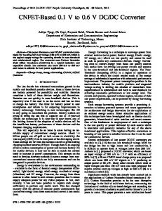
A well distinct plant (buck converter) is required for the controller design. The plant should be in its discrete form for the design of a discrete-time controller in direct digital design approach. The buck converter considering the DCR and ESR values of the inductor and capacitor respectively is shown in Fig. 1 in its circuit form. The converter converts 3.6 V to 2.0 V. For the design example, following values of the components are taken: C0 = 4.7 µF, L0 = 4.7 µH, rC = 5 mΩ, rL = 505 mΩ, R0 = 4.5 Ω, and fs = 1000 kHz. rL
Q1
L0 iL
iout rC R0
Vin C0
Q2
ZOH
Buck Converter
Vout
Digitized Plant
Discrete‐Time Controller
A/D Converter
Figure 1. A closed-loop buck converter system.
+
Abstract— The paper describes the optimization of a discretetime controller designed on the basis of discrete root locus for the boost converter operating at 1000 kHz. The optimization is accomplished through a nonlinear least squares method. The digital control theory is not as rich as the analog control theory. Locating poles and zeros directly in the z-plane by a designer to render the required performance is a difficult task to accomplish. Direct placement of poles and zeros may also introduce distortion as well. Consequently, direct digital design approach based digital controller may not offer satisfactory performance. The poles and zeros are disturbed around their nominal positions through the optimization technique to snub the atrocities introduced by the unwanted digital phenomena. Effect of nonlinearities in the form of ADC/DAC quantization error, delay, etc. on performance is also accentuated. The effectiveness of the application of the optimization technique to the buck converter is investigated using the MATLAB/Simulink environment.
Vref
The state space averaging and standard linearization technique suggested in [5] results in the following control-tooutput transfer function of the buck converter [6]:
⎡ Vin (s). ( rC Cs + 1) ⎤ G p (s) = ⎢ ⎥ Ψ (s) ⎢⎣ ⎥⎦
(1)
where ⎛L ⎞ ⎛ R +r ⎞ ⎛ R +r ⎞ Ψ (s) = L0 C0 ⎜ 0 C ⎟ s 2 + ⎜ 0 + rC C0 ⎜ 0 L ⎟ + rL C0 ⎟ s ⎜ ⎟ ⎝ R0 ⎠ ⎝ R0 ⎠ ⎝ R0 ⎠
(2)
⎛ R +r ⎞ +⎜ 0 L ⎟ ⎝ R0 ⎠
Using the zero-order-hold (ZOH) transformation technique with a sampling period of 1 µs, the buck converter is discretized as: ⎧⎪1 − e − sTs ⎫⎪ ⎪⎧ G p ( s ) ⎪⎫ Gp (z) = Ζ ⎨ .G p ( s ) ⎬ = 1 − z −1 .Ζ ⎨ ⎬ s ⎪⎩ s ⎭⎪ ⎩⎪ ⎭⎪
(
⇒ G p ( z ) = 0.080521.
(z
)
( z + 0.8643) 2
− 1.809 z + 0.8558
III.
Realizing the growing trend of digital control technology, digital controller based on the classical control theory, i.e., discrete root locus is designed [7]. Discrete root locus is quite analogous to analog root locus except the change in stability boundary from jω (s-plane) to the unit circle (z-plane). The procedure adopted here while designing the controller is highlighted as: •
The plant Gp(s) is discretized into its equivalent digital counterpart Gp(z) using some transformation techniques like zoh, foh, tustin, match, etc.
•
Corresponding to the required performance, a point in splane s0 is calculated using some specific values of damping ratio ζ, settling time ts, natural undamped frequency ωn, etc. For a standard second-order system, the overshoot and damping ratio are related by the formula:
(
(3)
(4)
)
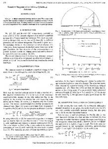
The digitized plant described in (4) clearly has one zero and two complex conjugate poles (see Fig. 2) lying close to the unit circle boundary which is an unstable area. The buck converter system thus requires compensation to pull the discrete-locus to pass through the desired point to effectuate the performance. The discrete lead compensator shifts the locus left towards the stable region to improve transient response. The lag compensator abolishes the steady-state error without disturbing transient characteristics. The conjugate poles will be compensated by the real-zeros of the compensator although complex zeros can also be used. 0.6π/T 0.8
0.5π/T
The desired point in s-plane is then mapped into the zplane by using the relation z = e sTs . Ts is the sampling period usually taken as the reciprocal of fs.
•
One of the poles of the plant is cancelled by one of the zeros of the compensator. The pole of the compensator is then calculated by fulfilling the phase angle condition, i.e., ∠G p ( z )Gc ( z ) =
-0.8
0.1 0.3π/T 0.2 0.3 0.4 0.2π/T 0.5 0.6 0.7 0.1π/T 0.8 0.9
0.8π/T
Imaginary Axis
0.9π/T
0.9π/T
•
•
The gain K of the compensator at the required point z0 is calculated by meeting the magnitude criterion, i.e.,
∏ z−z ( z )G ( z ) = K ∏ z− p
0.7π/T
0.3π/T 0.4π/T 0.5
Real Axis
Figure 2. Discrete root locus or pole-zero map of the buck converter.
c
i
=1
(7)
j
This completes the design of the lead portion of the compensator, i.e., Gcl ( z ) = K ( z − α ) ( z − β ) . If there exists some steady-state error, one additional pole and zero are placed near z = 1 such that z p > z z . For a type 0 system, placing a pole at z = 1 (integrator) removes the steady-state error fully.
0.2π/T
-0.5
(6)
j
• 0.8π/T
0.5π/T 0
j
j
= ±180 (2m + 1); m = 0, 1, 2,
0.1π/T
0.6π/T -1 -1
i
°
Gp
-0.4 -0.6
∑ ∠( z − z ) − ∑ ∠( z − p ) i
1π/T 0 1π/T -0.2
(5)
i
0.4 0.2
1 − ζ 2 π ⎤⎥ ⎦
•
0.4π/T
0.7π/T
0.6
)
M p (%) = 100.exp ⎡⎢ − ζ ⎣
Root Locus 1
DISCRETE-TIME CONTROLLER DESIGN
1
The step response is simulated to ensure the required performance by the discrete lead-lag controller.
For our design example, we set the overshoot of 16% giving the value of ζ = 0.6 using the relation (5). The bandwidth is set 10 times below the switching frequency while assuming ωn = ωB. The calculated desired point s0 = ( −3.77 ± 5.03i ) × 105 in s-plane, on knowing the value of ζ, ωn, and Ts, is mapped into the point z0 = 0.6011 ± 0.3304i in zplane using the mapping technique z = e sTs .
Following the procedure outlined above the discrete-time controller is given by:
⎛ z − 0.8047 ⎞ ⎛ z − 0.8047 ⎞ Gc ( z ) = 2.2766. ⎜ ⎟ .⎜ ⎟ ⎝ z − 0.1868 ⎠ ⎝ z − 1 ⎠
(8)
The step response shown in Fig. 3 offered by the discretetime controller demonstrates that the controller offers reasonable performance although there is an overshoot of 30.9%. Settling time is about 5.81×10⁻⁵s. The lead portion improves the transient response characteristics while the lag portion removes the steady-state error. The performance, however, can even further be improved by the nonlinear least squares method. Step Response 1.4
Vout (V)
2 2
represents the sum of squares of the error
signal. Lower and upper bounds on the design variables can also be imposed optionally to limit the solution always in the range lb ≤ x ≤ ub All this can be accomplished through the built-in MATLAB routine “lsqnonlin” which minimizes the sum of squares of the error, thus the error, while initially taking the nominal values of the discrete-time controller’s coefficients [8]. The routine ensures the well-tuned controller parameters for better set-point tracking. The lsqnonlin algorithm is of type large-scale as it exploits the linear algebra and does not require or store full matrices for its operation.
⎛ z − 0.8355 ⎞ ⎛ z − 0.8355 ⎞ Gc ( z ) = 13.0391. ⎜ ⎟ .⎜ ⎟ ⎝ z + 0.8795 ⎠ ⎝ z − 1 ⎠
1 0.8
0.4 0.2
0
1
2
3
4
5
6
7
8 -5
Time (seconds)
x 10
Figure 3. Step response of the compensated buck converter system.
The detail of the iterations along with monotonically decreasing value of f(x) while retuning the controller coefficients is shown in Fig. 4. The optimization process gets stopped when the relative change in the sum of squares becomes less than the selected value of the function tolerance.
IV.
THE NONLINEAR LEAST SQUARES OPTIMIZATION METHOD Optimization of the discrete-time controller is accomplished through nonlinear least squares (curve fitting) technique. It adjusts the controller coefficients in such a way that it minimizes the error e(t) between the output voltage Vout and the reference voltage Vref at all steps of the simulation time, thus constituting the multiobjective optimization problem. Actually it minimizes the sum of squares of the error signal, i.e.
min e( x) x
(12)
The routine, if observed minutely, makes teach the control designer to place the compensator real-zeros in the vicinity of plant poles and one of the compensator poles around the plant zero to cancel out the effect of each other rather than placing the compensator pole at 0.1868 as suggested by the classical digital controller in (8). Of course the other compensator pole (integrator) is placed at z = 1 to kill the steady-state error. This suggestion by the routine enormously ameliorates the performance.
0.6
0
The term e(x)
The discrete-time controller after the application of the optimization technique is given by:
Lead-Lag Lead
1.2
The vector x represents the number of design variables which are five in number (two poles, two zeros and a DC gain).
2 2
∑ e ( x) = min ( e ( x) + e ( x) = min x
x
2
i
i
1
2
2
2
+ … + en ( x)
2
)
(9)
subject to the constraints : ⎧⎪equality : Aeq .x = beq ⎨ ⎪⎩inequality : A.x ≤ b
(10)
where T
e( x) = ⎡⎣e1 ( x), e2 ( x),… , en ( x)⎤⎦ ⊃ ℜn
(11)
Figure 4. The nonlinear least squares method tuning results.
SIMULATION RESULTS
For the sake of comparing the performance offered by the traditional and optimized discrete-time controllers for the buck converter, MATLAB/Simulink environment is used. As can be noticed from the computer simulation results for the conventional discrete-time controller that the compensated buck converter system exhibits relatively more overshoots/undershoots and offers more settling and rise times. As a consequence, the nonlinear least squares optimization method is employed to fine-tune the discrete-time controller coefficients for the reduction of the overshoots/undershoots and the settling and rise times. Fig. 5 points towards the enormous improvement in performance through the optimized discretetime controller. Although the conventional discrete-time controller offers relatively better performance but the application of the nonlinear least squares optimization method to the conventional discrete-time controller enormously elevates the performance.
From the inspection of Fig. 6 and Fig. 7, it is depicted that the optimized compensated buck converter system keeps the output volatge regulated for the 50% change in load. The optimized controller compensates the changes in input volatge from 3.6 V to 4.6 V and then from 4.6 V to 3.6 V. Excellent load and line regulation is achieved. The nonlinearities introduce noise which can be observed on the output voltage waveform. The nonlinearities are within the acceptable range. As the delay is just half the µs, its effect on performance is not so much determental. 2.2 2.1 Vout (V)
V.
2 1.9 1.8 1.7 2.8
1.4 Taditional Optimized
1.2
3
3.2
3.4
3.6
3.8
4
4.2
4.4
4.6
4.8 -4
x 10 0.8 0.6
0.8
0.4
iL (A)
Vout (V)
1
0.2
0.6 0
0.4
-0.2 2.8
3
3.2
3.4
0.2
3.8 4 Time (sec)
4.2
4.4
4.6
4.8 -4
x 10
Figure 6. Load regulation offered by the optimized digital controller. 0.2
0.4 0.6 Time (sec)
0.8
1
Figure 5. Step response of the traditional and optimized digital controllers.
The comparison of performance with respect to rise time, settling time and percent overshoot is summarized in Table I. TABLE I.
3
-4
x 10
Vout (V)
0
PERFORMANCE OF CLASSICAL AND OPTIMIZED DIGITAL CONTROLLERS
Controller Traditional Controller Optimized Controller
Rise Time (s)
Settling Time (s)
2.37×10
-6
2.81×10
2.11×10
-7
-6
15×10
-5
2
1
0
0
0.1
0.2
0.3
0.4
0.5
0.6
0.7
0.8
0.9
Overshoot (%)
x 10
30.9
4.6
16.01
4.4
Uptill now, the load was fixed. No delays and quantizers were considered. In order to make the compensated system more realistic, the loop delay due to the conversion times taken by ADC and DAC and the processing time taken by the digital compensator is taken half of the switching period. The gains of the ADC and DAC are set equal to one for the sake of simplicity. The ADC and DAC quantizers are also included. The load and line regulation is investigated at cicuit-level through the optimized controller. PWM technique is employed to generate the duty cycle signal to derive the switches.
1 -3
Vin (V)
0
3.6
4.2 4 3.8 3.6
0
0.1
0.2
0.3
0.4
0.5 0.6 Time (sec)
0.7
0.8
0.9
Figure 7. Line regulation offered by the optimized digital controller.
1 -3
x 10
VI.
CONCLUSION
The strength of the paper lies in the optimization of discrete-time controller designed on the basis of discrete root locus. The sensitive poles and zeros are readjusted through the nonlinear least squares optimization method in such a way that the compensated system shows elevated performance. This reduces the burden of digital control designers to well-tune the controller coefficients. They just need to find the nominal values of the controller coefficients using the classical discretetime control theory. Rest is done by the nonlinear least squares optimization technique to fulfill the required static and dynamic performance. Compensation of the perturbations in load current and line voltage by the optimized discrete-time controller is also demonstrated. ADC and DAC quantizers and delays are introduced into the loop while ensuring excellent load/line regulation. The same procedure can be adopted to optimize the digital control of the other switching converters. Nonlinear minimization has been accomplished through “Trust-Region Method” which can be exploited by Gauss-Newton method to enhance efficiency. Other advanced numerical methods based optimization techniques can also be tested and compared performance-wise. Hardware implementation of the suggested compensated buck converter system is the task that can be accomplished in future.
REFERENCES [1]
[2]
[3]
[4]
[5]
[6]
[7]
[8]
Y. Duan and H. Jin, “Digital Controller Design for Switchmode Power Converters”, IEEE Applied Power Electronics Conference 1999, vol. 2, March 1999, pp. 967–973. Liu, Yan-Fei, Eric Meyer, and Xiaodong Liu. "Recent developments in digital control strategies for DC/DC switching power converters." Power Electronics, IEEE Transactions on, vol. 24, no. 11 (2009): 2567-2577. Buccella, Concettina, Carlo Cecati, and Hamed Latafat. "Digital control of power converters—A survey." Industrial Informatics, IEEE Transactions on, vol. 8, no. 3 (2012): 437-447. Qahouq, Abu, and V. Arikatla. "Online closed-loop autotuning digital controller for switching power converters." Industrial Electronics, IEEE Transactions on, vol. 60, no. 5 (2013): 1747-1758. R. D. Middlebrook and S. Cuk, “A General Unified Approach to Modeling Switching-Converter Power Stages,” IEEE Power Electronics Specialists Conference (PESC), 1976, pp. 18–34. B. Johansson, “DC-DC Converters, Dynamic Model Design and Experimental Verification,” Dissertation LUTEDX/(TEIE-1042)/1194/(2004), Dep. of Industrial Electrical Engineering and Automation, Lund University, Lund, 2004. Rolf Isermann, “Digital Control Systems: Volume 1: Fundamentals, Deterministic Control”, Springer Science & Business Media, ISBN: 3642864171, 9783642864179, 2013. Coleman, Thomas, Mary Ann Branch, and Andrew Grace. Optimization Toolbox for Use with MATLAB: User's Guide, Version 7.1. Math Works, Incorporated, 2013.