Closed-Loop Statistical Verification of Stochastic Nonlinear Systems ...

Closed-Loop Statistical Verification of Stochastic Nonlinear Systems Subject to Parametric Uncertainties

arXiv:1709.06645v1 [cs.SY] 19 Sep 2017

John F. Quindlen1

Ufuk Topcu2

Abstract— The increasing adoption of complex, nonlinear control techniques motivates the development of new statistical verification methods for efficient simulation-based verification analysis. The growing complexity of the control architectures and the open-loop systems themselves limit the effective use of provable verification techniques while general statistical verification methods require exhaustive simulation testing. This paper introduces a statistical verification framework using Gaussian processes for efficient simulation-based certification of stochastic systems with parametric uncertainties. Additionally, this work develops an online validation tool for the identification of parameter settings with low prediction confidence. Later sections build upon earlier work in closed-loop deterministic verification and introduce novel active sampling algorithms to minimize prediction errors while restricted to a simulation budget. Three case studies demonstrate the capabilities of the validation tool to correctly identify low confidence regions while the new closed-loop verification procedures achieve up to a 35% improvement in prediction error over other approaches.

I. I NTRODUCTION Ever increasing demands for high performance necessitates the adoption of advanced, nonlinear control techniques in a wide variety of engineering systems. The complexity of these control architectures, coupled with the increasing complexity of the open-loop systems themselves, complicates certification that the closed-loop system actually satisfies the performance requirements at off-nominal conditions, labeled parametric uncertainties. Control system verification analyzes the closed-loop system and attempts to identify at which parametric uncertainties the resulting trajectory fails to meet the requirements. Traditional analytical and numerical verification techniques [1], [2] provably certify the behavior of the system at various uncertainties, but large state and parameter spaces, highly nonlinear dynamics, and hybrid control architectures impair their suitability in complex systems. Recent work [3]– [5] addressed some of these concerns, but their utility is still limited in complex nonlinear systems. Stochastic dynamics further challenge these approaches and restrict their suitability. For comparison, statistical verification techniques [6], [7] replace provable guarantees with looser probabilistic bounds, but are capable of handling a much broader range of problems with fewer restrictions. Statistical verification 1 Ph.D.

Candidate, Department of Aeronautics and Astronautics, Massachusetts Institute of Technology (MIT). 2 Assistant Professor, Department of Aerospace Engineering and Engineering Mechanics, University of Texas at Austin 3 Assistant Professor, Departments of Agricultural & Biological Engineering and Aerospace Engineering, University of Illinois Urbana-Champaign 4 Richard C. Maclaurin Professor of Aeronautics and Astronautics, Laboratory for Information and Decision Systems (LIDS), MIT

Girish Chowdhary3

Jonathan P. How4

methods rely upon extensive simulations of the system to test the likelihood of requirement satisfaction at various conditions and are well-suited to stochastic systems. Recent work developed data-driven statistical verification techniques [8], [9] to efficiently verify closed-loop systems without relying upon exhaustive simulations. These deterministic methods construct machine learning models from small sets of simulation trajectories and predict the response at unobserved parameter settings. The latest work [10] introduced Gaussian process (GP) prediction models and novel active sampling procedures to improve the accuracy of predictions given limited amounts of simulation data. The deterministic GP-based approach also quantifies the prediction confidence online without the need for external validation datasets and carefully selects simulations to maximize the prediction confidence. This paper extends data-driven methods to stochastic verification problems and provides three primary contributions. First, Section III presents a stochastic statistical verification framework to predict the probability of requirement satisfaction at all possible parametric uncertainties. This GPbased framework infers the underlying satisfaction probability function from nondeterministic simulations at different parameter settings. Additionally, Section III-B introduces a novel validation tool for online identification of regions with low prediction confidence. Reformulated active sampling procedures in Section IV exploit this new validation metric and iteratively minimize prediction error to create a closedloop verification process. Three case studies at the end demonstrate the effectiveness of the paper’s contributions for resource-constrained statistical verification. II. P ROBLEM D ESCRIPTION Consider the closed-loop nonlinear system ˙ x(t) = fcl (x(t), θ, w(t)) p

(1)

subject to parametric uncertainties θ ∈ R , where x(t) ∈ Rn is the state vector. Since the goal is to verify the suitability of a candidate control policy, this work specifically examines the closed-loop dynamics after the candidate control policy has been added to the open-loop system. This control policy will generate control inputs u(t) ∈ Rm for the open-loop system according to some predetermined strategy. The closed-loop dynamics are a function of parametric uncertainties θ which can arise from a variety of sources. For instance, these parameters may include uncertainties about the initial state x(0) or other system properties such as vehicle mass and inertia that will typically vary across

different operational scenarios. Note that the nominal initial state vector x0 is assumed to be known and fixed and any uncertainties (x(0) 6= x0 ) are treated as perturbations to x0 , i.e. x(0) = x0 +θ. The main impact of the parametric uncertainties is as uncertain initial conditions that determine the evolution of the subsequent state trajectory. These parametric uncertainties may not be known during real-world execution of the system, but are assumed to fall within some bounded, compact set Θ that is known in advance. Assumption 1 The set of all possible parametric uncertainties θ ∈ Θ is a known, compact set Θ ∈ Pp . Assumption 1 ensures the system has known feasible bounds on the uncertain conditions for the verification procedure to examine. Most physical systems will naturally have bounds on the set of allowable operating conditions. For instance, aircraft will typically fly within a maximum take-off weight set by structural limitations and a minimum (empty) weight. The major difference between (1) and earlier problems [8]–[10] is the addition of nondeterministic noise w(t) in the dynamics. This noise term encapsulates any source of nondeterminism such as process and/or measurement noise and ultimately breaks the previous works’ fundamental assumption of deterministic (noise-free) dynamics. Multiple simulations of the system starting from the same nominal x0 and perturbation vector θ will each produce different closedloop trajectories Φ(x(t)|x0 , θ) due to the stochasticity. Not surprisingly, this randomness will have a potentially large effect upon the satisfaction of the performance requirements at a given x0 and θ. A. Measurements of Trajectory Performance The closed-loop trajectory must meet certain performance requirements in order for trajectory Φ(x(t)|x0 , θ) to be considered “satisfactory.” As before [10], these requirements are supplied by relevant certification authorities and may include a wide range of potential specifications with varying complexity. This work assumes the simulation model indicates the robustness of a completed trajectory Φ(x(t)|x0 , θ) to a given performance requirement with a single measurement variable y(θ). Assumption 2 The simulation model provides a single, scalar output y(θ) ∈ R that measures the minimum robustness of trajectory Φ(x(t)|x0 , θ) to a specified performance requirement. The sign of y(θ) indicates satisfaction of the requirements, where positive y > 0 signifies “satisfactory” performance and y ≤ 0 signifies “unsatisfactory” performance. Since the closed-loop trajectory is a function of nominal (fixed) x0 and parameters θ, we write the trajectory robustness measurements y(θ) as an explicit function of θ to emphasize the effect of the parametric uncertainties upon the robustness of the trajectory. As θ changes, so will the satisfaction of the performance requirement.

Different applications will produce robustness measurements y(θ) through various mean. For example, signal temporal logic (STL) [11] is a widely-used mathematical framework for modeling the requirements with temporal logic specifications. Central to this framework is the computation of a scalar robustness degree ρϕ ∈ R that quantifies the minimum robustness of a trajectory with respect to a set of temporal logic specifications ϕ (the requirement) and is an obvious potential source for measurement y(θ). Other applications will quantify the satisfaction of the performance requirements through different methods like realized reward or score functions, as will be seen in the task allocation example from Section V-B. B. Probabilistic Satisfaction of Requirements Although the trajectory and its corresponding robustness measurement are functions of parametric uncertainties, stochasticity causes multiple trajectories at the same θ setting to obtain different y(θ). As the number of repetitions grows, these measurements quickly define a continuous distribution of possible robustness values at every θ ∈ Θ. The underlying true distribution of y(θ) may take a variety of different forms, but this work addresses the baseline case with a simple Gaussian distribution. Assumption 3 The distribution of robustness measurements y(θ) at every θ follows a Gaussian distribution y(θ) ∼ N (¯ y (θ), 2y ) with spatially-varying mean y¯(θ) and constant standard deviation y . While this assumption does restrict the class of problems, this paper lays the groundwork for a more complex framework able to handle non-Gaussian distributions. Upcoming work will relax Assumption 3 and present extensions to this paper’s baseline approach for spatially-varying noise and non-Gaussian distributions. From the verification perspective, where each trajectory either satisfies the requirement or does not, the Gaussian distribution of y(θ) creates a Bernoulli distribution for the likelihood an arbitrary trajectory at θ will satisfy the requirement. Definition 1 The satisfaction probability function psat (θ) ∈ [0, 1] defines the probability an arbitrary trajectory initialized with θ will satisfy the performance requirement. This probability of satisfaction is the cumulative distribution of positive y(θ) measurements,   y¯(θ) 1 1 . (2) psat (θ) = P(y(θ) > 0) = + erf q 2 2 22y While psat (θ) defines the probabilistic satisfaction of the requirements, the challenge for stochastic verification is psat (θ) will generally be unknown in advance. Instead, the statistical verification goal is to predict psat (θ) for all possible conditions in Θ. Likewise, the verification process

must also contend with computational costs. It may seem straightforward to simply saturate Θ with simulations, but the complexity of the simulation model or other factors impart a computational budget on statistical verification. This work models the computational budget as a feasible upper bound Ntotal on the number of simulation trajectories. The complete statistical verification problem is summarized below. Problem 1 Given a stochastic closed-loop simulation model (1), compute the estimated satisfaction probability function pbsat (θ) given a limited number of simulation trajectories, Ntotal . III. S TATISTICAL V ERIFICATION F RAMEWORK Given the objective in Problem 1, there are multiple possible approaches to compute pbsat (θ) from a finite set of simulation-based observations. The most basic form is to treat each trajectory as a Bernoulli trial with binary evaluations {“satisfactory”, “unsatisfactory”} from the sign of y(θ). While this approach can address all types of systems, including those that do not meet Assumptions 2 and 3, a binary-based approach requires multiple trials at every θ ∈ Θ to construct a binomial distribution. Instead, this work entirely avoids the need for expensive binomial distributions in the relevant class of systems through the direct use of y(θ) and its Gaussian probability density function (PDF). The main idea is to exploit a single stochastic trajectory at each training location and its noisy measurement y(θ) to infer the underlying PDF, which defines the cumulative distribution psat (θ). Although various computational methods are possible [12], [13], this problem is particularly well-suited to Gaussian process regression [14]. A. GP-based Prediction Model The Gaussian process regression model follows a similar format to the earlier work in verification of deterministic systems [10]. A finite collection of N total simulation trajectories forms a training dataset L = {D, y} consisting of their parameter settings D = {θ 1 , θ 2 , . . . , θ N } and corresponding robustness values y = [y(θ 1 ), y(θ 2 ), . . . , y(θ N )]T . Unlike the deterministic approach, these noisy measurements require the introduction of a Gaussian likelihood model where the GP does not model y(θ) directly, but infers the latent mean y¯(θ). The training process constructs the GP regression model from the information provided by the training dataset L. More details are found in [14], but fundamentally the training procedure uses Bayesian inference to place a pos¯ given L. terior probability distribution on latent mean y Assuming a zero-mean prior N (¯ y|0, K) and likelihood model N (y|¯ y, 2y I), the posterior predictive distribution at an arbitrary location θ ∗ follows a Gaussian distribution P(¯ y(θ ∗ )|L, θ ∗ ) = N (µ(θ ∗ ), Σ(θ ∗ )). The posterior predictive mean µ(θ ∗ ) and covariance Σ(θ ∗ ) are given by
−1 µ(θ ∗ ) = KT∗ K + 2y I y (3)
−1 T Σ(θ ∗ ) = κ(θ ∗ , θ ∗ ) − K∗ K + 2y I K∗ ,

where κ(θ i , θ j ) is the scalar kernel function, K∗ is the N ×1 vector of κ(θ ∗ , θ i ) ∀i = 1 : N and K is the N × N matrix for κ(θ i , θ j ) ∀i, j = 1 : N . Different choices are possible, but this work uses the common squared exponential kernel with automatic relevance determination (SE-ARD) [14] for the kernel function. The choice in GP hyperparameters may drastically change the predictive distribution, even with the same training set L, since these hyperparameters control the kernel function κ(., .) and the likelihood model. Unfortunately, the ideal/true choice of hyperparameters that perfectly replicates y¯(θ) will not be known in advance and must be estimated online. This work uses maximum likelihood estimation (MLE) [14] to optimize the kernel hyperparameters given only the information provided by L. The use of the SE-ARD kernel also enables the MLE procedure to adjust the sensitivity of the kernel to each element of θ as y¯(θ) may have a higher sensitivity to certain elements than others. Additionally, the likelihood model contains a hyperparameter to estimate standard deviation y as this term may also be completely unknown. If y is unknown, then estimate b y may be computed in the same MLE optimization process as the kernel hyperparameters or separately by repeated sampling at a training locations in D. 1) Expected Probability of Satisfaction: Although µ(θ ∗ ) and Σ(θ ∗ ) define the predictive PDF for y¯(θ ∗ ), (3) only completes half the goal. Problem 1 requires the cumulative distribution function (CDF) for y(θ ∗ ), not the PDF. The CDF in (2) defined the true psat (θ), but this computation requires perfect knowledge of y¯(θ) (and y ). Instead, the predicted satisfaction probability function pbsat (θ) marginalizes the CDF over the posterior predictive distribution of y¯(θ), h
i y (θ ∗ ) pbsat (θ ∗ ) = Ey¯(θ∗ ) P y(θ ∗ ) > 0|¯   µ(θ) 1 1 (4) . = + erf q 2 2 2(Σ(θ ∗ ) + 2y ) This result provides the stochastic verification framework’s solution to Problem 1. B. Prediction Confidence While (4) computes the expected probability of requirement satisfaction, pbsat (θ) will likely fail to perfectly model psat (θ). Therefore, the statistical verification framework must not only provide pbsat (θ), but also indicate where its confidence in the accuracy of these predictions is low. Unsurprisingly, the true prediction error pesat (θ) = psat (θ)− pbsat (θ) is unknown, but offline validation methods using external validation datasets [12] can estimate pesat (θ) by comparing the predictions against the validation set’s known, true values. However, these external validation methods are wasteful as they generally require the removal of valuable training data for the independent validation set. For comparison, probabilistic inequalities provide theoretically-justified bounds on pesat (θ) without the use of validation sets. In particular, Chebyshev’s inequality bounds

the prediction error by the variance of the CDF, h
i Vy¯(θ∗ ) P y(θ ∗ ) > 0|¯ y (θ ∗ ) , (5) P(|e psat (θ)| ≥ a) ≤ a2 where a > 0. Lower variance Vy¯(θ∗ ) [. . .] will translate into lower probabilistic bounds on pesat (θ) and thus higher confidence in the accuracy of pbsat (θ). The primary challenge with (5) is the variance lacks an analytical closed-form solution. Fortunately, the variance can be approximated using a 1st or 2nd order Taylor series expansion of the nonlinear random function [15]. The 1st order approximation is   1 −µ(θ∗ )2 /2y e Σ(θ ∗ ), Vy¯(θ∗ ) P(y(θ ∗ ) > 0|¯ y (θ ∗ )) ≈ 2π2y (6) which also happens to always upper bound the 2nd order approximation. For simplicity, we subsequently refer to the approximate CDF variance in (6) as V (θ|L). Despite the convenience of (6), the accuracy of an approximation of a nonlinear random function is limited. This inaccuracy makes it inadvisable to blindly substitute (6) into (5) without careful consideration. However, the approximation in (6) does still provide a perfect metric to identify regions of Θ where the confidence in pbsat (θ) is low and provide intuition on the sensitivity of pesat (θ). The power of (6) is its value as a computationally-efficient, online validation tool for signifying prediction confidence. For instance, approximate variance is highest in regions with µ(θ) ≈ 0 and Σ(θ) > 0, meaning the confidence in the predictions should be quite low. The next section will exploit the approximate CDF variance to derive a closed-loop verification process in order to minimize prediction errors. IV. C LOSED -L OOP S TATISTICAL V ERIFICATION In many applications, external constraints restrict the computational budget allocated to the statistical verification process. For instance, verification testing often relies upon high-fidelity models of complex systems and subsystems that drive up the computational time for a single trajectory. Regardless of the source, each application has some feasible limit on the amount of time, resources, or money allocated to testing. Problem 1 approximated this limit as a cap on the number of simulation trajectories, |L| ≤ Ntotal . Given this restriction on the size of training dataset L, the ideal scenario would only perform informative simulations and carefully select all θ ∈ D to minimize the prediction error at all θ ∈ Θ. However, the information-maximizing training dataset is not apparent until after all the trajectories have been obtained. To address that issue, this work applies active learning [16] to iteratively select informative θ settings for future simulation trajectories and minimize the expected prediction error. To emphasize the iterative, feedback-based nature of the active learning procedure, we label the process closed-loop statistical verification. Active learning describes a wide variety of different procedures [16]–[21], each with their own definition for the “best” sample to run next. Most of these procedures focus on a

particular aspect of the Gaussian PDF. For instance, PDF mean-focused procedures [9], [17] favor points with y¯(θ) near zero, meaning the best location is θ = argmin|µ(θ)|. Although originally intended for binary classification with support vector machines, such an approach does correctly label points with µ(θ) ≈ 0 as informative since the CDF variance (6) is high there. Likewise, PDF variance-based approaches and extensions [18]–[21] are significantly more common for GP methods and aim to reduce the PDF variance Σ(θ). These approaches favor points with high variance, θ = argmax Σ(θ), which also correctly emphasizes points with comparatively high CDF variance since Σ(θ) >> 0. Although they both correctly emphasize certain aspects, neither of those two approaches explicitly minimize the posterior CDF variance. A. Reduction in CDF Variance Earlier work in deterministic closed-loop verification [10] specifically developed new sample selection metrics to maximize prediction confidence. Even though the implementation details have changed, this work utilizes the same underlying motivation and attempts to minimize the approximate CDF variance (6) in order to maximize the confidence in pbsat (θ). The ideal selection criteria would minimize the maximum posterior CDF variance V (θ|L+ ) after the new sample data at θ was added, but this requires the posterior training set L+ = L∪{θ, y(θ)} to be known apriori. Prior knowledge of L+ is an impossible proposition since y(θ) cannot be known before a simulation has actually been performed there. Even if the expected posterior set Lb+ = L ∪ {θ, µ(θ)} replaces infeasible L, the high computational cost of retraining the GP at every prospective sample location, nominally an O(N 3 ) operation and O(N 2 ) at best, renders the approach computationally intractable. A more computationally tractable approach maximizes the local improvement in posterior CDF variance, effectively selecting the θ condition which will experience the greatest reduction in CDF variance if a sample is taken at that location. The local change in CDF variance is labeled by Ve (θ|L) = V (θ|L)−V (θ|Lb+ ). Although the change Ve (θ|L) requires expected posterior information Lb+ , it does not require the GP model to be retrained, which was the source of the previous computational intractability. The local posterior CDF variance at location θ ∗ after a measurement there can be written purely in terms of the current information. After the Woodbury matrix identity, the expected posterior covariance Σ(θ ∗ )+ reduces to  Σ(θ ∗ )  Σ(θ ∗ )+ = Σ(θ ∗ ) 1 − (7) Σ(θ ∗ ) + 2y while mean µ(θ ∗ )+ = µ(θ ∗ ). Ultimately, the local change in CDF variance is given by   1 −µ(θ∗ )2 /2y Σ(θ ∗ ) Σ(θ ) Ve (θ ∗ |L) = e . (8) ∗ 2π2y Σ(θ ∗ ) + 2y Note that the CDF variance reduction criteria in (8) favors points with µ(θ) ≈ 0 and Σ(θ) >> 0, just as in (6).

B. Sampling Algorithms The section criteria from (8) forms the basis of the closedloop stochastic verification framework. Since the actual space Θ is infinite, the framework constructs a high resolution lattice Θd to replicate Θ and then selects all samples from Θd rather than Θ directly (D ⊂ Θd ). Set U = Θd \ D contains all remaining points not in training set L available for future simulations. This paper presents two versions of the closed-loop verification framework. 1) Sequential Sampling: The most straightforward implementation of closed-loop verification is sequential sampling, described in Algorithm 1. The process first starts with an initial training set L of passively-selected samples, usually obtained through random sampling or another open-loop design of experiments approach. This initial training set of size |L| = N0 produces the initial GP so active sampling can be performed. The sequential procedure then selects one sample from U according to (8) before it performs one simulation at the selected θ condition, obtains y(θ), and updates the GP prediction model. This iterative procedure repeats until the number of remaining samples T = Ntotal − N0 has been reached. Algorithm 1 Sequential closed-loop stochastic verification Input: initial training set L = {D, y}, available sample locations U, max # of additional samples T 2: Initialize: train GP regression model 3: for i=1:T do 4: Select θ = argmax Ve (θ|L) 1:

θ∈U

Perform test at θ, obtain measurement y(θ) Add {θ, y(θ)} to training set L, remove θ from U Retrain GP model with updated L 8: end for
9: Return: expected p bsat (θ) and variance V θ|L

5: 6: 7:

2) Batch Sampling: In comparison to Algorithm 1, batch sampling [16] offers further computational efficiency by selecting multiple samples between retraining steps. Assuming the same limit Ntotal , batch selection reduces the number of GP retraining processes and can also fully exploit any parallel computing capabilities of the simulation environment. Batch approaches select M samples at once and perform their simulations in parallel. While this provides computational savings, it also introduces the possibility of redundant samples if the batch sample set S does not possess adequate diversity. First proposed for deterministic closed-loop verification in [10], determinantal point processes (DPPs) [22] present efficient probabilistic methods for encouraging diversity within S without severe computational overhead. The batch framework first converts Ve (θ|L) into a probability distribution PV (θ) = Ve (θ|L)/ZV , where ZV is the normalization constant. A relatively small number of MT samples are obtained from Θd according to PV (θ) and used to construct a DPP. This paper uses MT = 1000, but these are simply

samples of θ locations from the distribution and no actual simulations are performed. The DPP randomly selects M locations for S based upon a modified version of PV that penalizes similarities in S and subsequently spreads the datapoints out across high-valued regions in Θd with significantly less redundancy. Algorithm 2 details the batch closed-loop verification framework. Rather than T number of additional samples, Algorithm 2 operates in T batches of M samples, assuming M × T ≤ Ntotal − N0 . Algorithm 2 Batch closed-loop stochastic verification framework using determinantal point processes 1: 2: 3: 4: 5: 6: 7: 8: 9: 10: 11: 12:

Input: initial training set L = {D, y}, available sample locations U, # of iterations T , batch size M Initialize: train GP regression model for i=1:T do Initialize: S = ∅ Transform Ve (θ|L) into distribution PV (θ) Form k-DPP from MT random samples of PV (θ) Generate M random samples from DPP, add to S Perform tests ∀θ ∈ S, obtain measurements yS Add {S, yS } to training set L, remove S from U Retrain GP model with updated L end for
Return: expected pbsat (θ) and variance V θ|L V. E XAMPLES

This section examines statistical verification applied to three stochastic systems and demonstrates the improved performance of Algorithms 1 and 2 over existing techniques. A. Example 1: Model Reference Adaptive Control System The first example considers a stochastic version of the concurrent learning model reference adaptive control (CLMRAC) system from earlier deterministic work [9], [10]. The CL-MRAC example examines a second order linear system with two uncertain parameters θ = [θ1 , θ2 ]T . The adaptive control system estimates these parameters online and attempts to track a desirable reference trajectory. The nonlinearities associated with adaptation result in a highly nonlinear closed-loop system. The verification goal is to predict the probability the actual trajectory will remain within 1 unit of the reference trajectory at all times between 0 ≤ t ≤ 40 seconds, given in STL format as ϕ = [0,40] (1 − |e1 [t]| ≥ 0) (9) where tracking error e1 (t) is the difference between actual position x1 (t) and reference position xm1 (t). Measurement y(θ) is the STL robustness degree ρϕ for the trajectory initialized with uncertainty setting θ. The sampling lattice Θd covers θ1 : [−10, 10] and θ2 : [−10, 10] with a grid of 40,401 points. In this example, the open-loop dynamics are subject to additive process noise with Gaussian distribution w(t) = N (0, diag(1, 1)). The underlying true distribution was obtained by repeated sampling at each of the points

24 Open-Loop PDF Mean PDF Variance CDF Variance

10 8 6 4 2 0

22 20

Open-Loop PDF Mean PDF Variance CDF Variance

18 16 14 12 10

100

200

300

400

# Samples

100

50 Open-Loop PDF Mean PDF Variance

0 100

200

300

100

200

300

400

# Samples

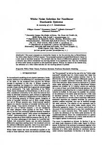
Fig. 1: (Example 1) Comparison of mean absolute error (MAE) convergence for the four different sampling strategies. The standard deviation intervals around the mean (solid lines) are given by the 0.5σ bound.

Outperforms (%)

Perecent Improvement (%)

Mean Absolute Error (%)

12

400

# Samples

Fig. 2: (Example 1) Ratio of tests where Algorithm 2 directly outperforms the indicated strategies.

Fig. 3: (Example 1) Reduction in MAE after all points with the top 5% of CDF variance are removed.

the true CDF variance is unavailable, but the approximate CDF variance (6) still provides a meaningful metric to compare prediction confidence across Θd . One of the best uses of (6) is to rank points in Θd according to their CDF variance in order to identify which predictions to trust the least. Figure 3 displays the reduction in prediction error when the points with the top 5% of CDF variance are removed. The 12-22% improvement in MAE proves that the CDF variance did indeed correctly identify and remove regions with large pesat (θ). When the top 10% are removed, the MAE improvement jumps to 40%. B. Example 2: Robust Multi-Agent Task Allocation

in Θd . To avoid any potential issues, Gaussian distributions were fit to the raw data and the variance was averaged across Θd to return y = 0.0372. Figure 1 compares the performance of Algorithm 2 against similar procedures using the existing selection metrics discussed in Section IV as well as an open-loop, random sampling procedure. These procedures all start with an initial training set of 50 observations and select batches of M = 10 points until a total of 450 simulations has been reached. Neither the kernel hyperparameters nor y are assumed to be known so the procedures estimate these online using maximum likelihood estimation. In order to fairly compare each procedure, the algorithms all start from the same 100 randomly-chosen initial training sets with the same random seed. At the conclusion of the process, Algorithm 2 demonstrates a 29%, 31%, and 35% improvement in average mean absolute error (MAE) over the PDF mean, PDF variance, and random sampling approaches. Additionally, the performance of the algorithms in each of the 100 test cases can be directly compared since they all start with the same L and random seed. At this level, Figure 2 illustrates that Algorithm 2 either matches or outperforms the existing sampling strategies eventually nearly 100% of the time. Although the exact numbers will change for different distributions, these results highlight the value of the selection criteria from (8) to further reduce prediction error given a fixed number of samples. Figure 3 demonstrates the utility of CDF variance to identify regions of large prediction errors, regardless of the particular sampling strategy. As discussed in Section III-B,

The second example addresses the robust multi-agent task allocation problem from [23] with added stochasticity. The task allocation problem attempts to assign a team of four UAVs to complete fire surveillance tasks that will take longer or shorter depending on the wind speed θ1 and direction θ2 . Task durations are also corrupted by zero-mean Gaussian noise. Unforeseen time delays will compound and may potentially lead the UAVs to miss the completion of tasks within their assigned window, thus lowering the overall realized mission score. The verification goal is to determine whether the team of UAV agents will sufficiently complete the ordered tasking and achieve a minimum mission score at different wind settings. Sampling grid Θd spans the set of feasible wind conditions θ1 : [0◦ , 359◦ ], θ2 : [0, 40] km/hr with 16,641 possible trajectory settings. Figures 4 and 5 compare the performance of Algorithm 1 against the competing sampling strategies. Ultimately, the MAE performance is consistent with the last example. Algorithm 1 demonstrates a 10-20% improvement in average MAE over the existing strategies and either matches or exceeds the MAE of the competing approaches when directly compared against one another. Figure 6 demonstrates a similar reduction in MAE as witnessed in Figure 3. Once the points with the top 5% of CDF variance are removed, the MAE of the predictions in the remaining 95% of the data reduces by up to 12-16%. If the top 10% are removed, the average reduction reaches at least 28% for all the sampling strategies. This supports

10 Open-Loop PDF Mean PDF Variance CDF Variance

15

Mean Absolute Error (%)

Mean Absolute Error (%)

20

10

Open-Loop PDF Mean PDF Variance CDF Variance

9 8 7 6 5 4

5 20

30

40

50

60

70

80

3 100

90

200

300

400

500

# Samples

# Samples

Fig. 4: (Example 2) Comparison of MAE convergence for the four different sampling strategies over 250 randomly selected initializations.

Fig. 7: (Example 3) Comparison of MAE convergence for the four different sampling strategies over 90 random initializations. Outperforms (%)

Outperforms (%)

100 100

50 Open-Loop PDF Mean PDF Variance

30

40

50

60

70

80

90

Perecent Improvement (%)

Fig. 5: (Example 2) Ratio of tests where Algorithm 1 directly outperforms the indicated strategies. 18 16 14 12 Open-Loop PDF Mean PDF Variance CDF Variance

8 6 20

30

40

50

60

70

80

90

# Samples

Fig. 6: (Example 2) Reduction in MAE after all points with the top 5% of CDF variance are removed.

the conclusion that CDF variance identifies points with low prediction confidence where pesat (θ) may be large. C. Example 3: Lateral-Directional Autopilot Lastly, the third example considers the altitude-hold requirement of a lateral-directional autopilot [24]. In this problem, a Dryden wind turbulence model [25] augments the original nonlinear aircraft dynamics model to introduce stochasticity into the closed-loop dynamics. The performance requirement expects the autopilot to maintain altitude x(t) within a set threshold of the initial altitude when the autopilot is engaged. This work explores a relaxed version of the original requirement [24] in which the aircraft must remain within a 55 foot window around the initial altitude x(0), ϕ = [0,50] (55 − |x[t] − x[0]| ≥ 0).

200

300

400

500

# Samples

# Samples

10

Open-Loop PDF Mean PDF Variance

0 100

0 20

50

(10)

The performance measurement is the STL robustness degree ρϕ . This example tests the satisfaction of the requirement against initial Euler angles for roll θ1 : [−60◦ , 60◦ ], pitch

Fig. 8: (Example 3) Ratio of tests where Algorithm 2 directly outperforms the indicated strategies.

θ2 : [4◦ , 19◦ ], and yaw θ3 : [75◦ , 145◦ ] with a constant reference heading of 112◦ . The 3D grid Θd consists of 524,051 possible sample locations. Figures 7 and 8 illustrate the MAE performance of the four different sampling strategies given a batch size of M = 10. The equivalent of Figures 3 and 6 is skipped but displays the same exact behavior. This example begins with 100 samples in the initial training set L and compares the performance over 90 random initializations. As before, Algorithm 2 outperforms the PDF variance-focused and random sampling procedures with a 29% reduction in average MAE. Unlike the previous two examples, Algorithm 2 only slightly edges out the competing mean-focused strategy. This new result is due to the comparatively low y for noisy y(θ) from the lowaltitude turbulence model. The resulting tighter distribution only experiences changes in psat (θ) near y¯(θ) = 0, which favors the mean-focused selection criteria. If the turbulence is increased then the distribution widens dramatically and the performance of the PDF mean-focused metric degrades significantly like the previous two examples. These case studies all highlight the improved performance of the novel CDF variance algorithms compared to the existing sampling strategies. Just as important, Algorithms 1 and 2 will remain the best even as the distribution changes, whereas the other strategies will trade positions according to changes in y . VI. C ONCLUSION This work introduced machine learning methods for simulation-based statistical verification of stochastic nonlinear systems. In particular, the paper presented a GP-based statistical verification framework to efficiently predict the

probability of requirement satisfaction over the full space of possible parametric uncertainties given a limited amount of simulation data. Additionally, Section III-B developed new criteria based upon the variance of the cumulative distribution function to qualify confidence in the predictions. This metric provides a simple validation tool for online identification of regions where the prediction confidence is low. Section IV builds upon this metric and introduces sequential and batch sampling algorithms for efficient closedloop verification. These new verification procedures demonstrate up to a 35% improvement in prediction error over competing approaches in the three examples in Section V. The examples also serve to highlight the utility of the CDF variance to correctly identify low-confidence regions in the parameter space without external validation datasets. While the paper only considers Gaussian distributions for the performance measurements, this work lays the foundation for more complex statistical verification frameworks capable of handing a wider range of distributions. Upcoming work will adapt the CDF variance metric and closed-loop verification procedures to recent developments in modeling of spatially-varying standard deviations [26] and non-Gaussian distributions [27]. Additionally, this work can be extended to high-dimensional GP representations [28]. While the implementation considers Gaussian distributions, this paper’s underlying concepts have broader utility. R EFERENCES [1] E. M. Clarke, O. Grumberg, and D. A. Peled, Model Checking. MIT Press, 1999. [2] S. Prajna, “Barrier certificates for nonlinear model validation,” Automatica, vol. 42, no. 1, pp. 117–126, 2006. [3] U. Topcu, “Quantitative local analysis of nonlinear systems,” Ph.D. dissertation, University of California, Berkeley, 2008. [4] A. Majumdar, A. A. Ahmadi, and R. Tedrake, “Control and verification of high-dimensional systems with DSOS and SDSOS programming,” in IEEE Conference on Decision and Control, 2014. [5] J. Kapinski, J. Deshmukh, S. Sankaranarayanan, and N. Arechiga, “Simulation-guided Lyapunov analysis for hybrid dynamical systems,” in Hybrid Systems: Computation and Control, 2014. [6] P. Zuliani, C. Baier, and E. M. Clarke, “Rare-event verification for stochastic hybrid systems,” in Hybrid Systems: Computation and Control, 2012. [7] E. M. Clarke and P. Zuliani, “Statistical model checking for cyberphysical systems,” in International Symposium for Automated Technology for Verification and Analysis, 2011. [8] A. Kozarev, J. F. Quindlen, J. P. How, and U. Topcu, “Case Studies in Data-Driven Verification of Dynamical Systems,” in Hybrid Systems: Computation and Control, 2016.

[9] J. F. Quindlen, U. Topcu, G. Chowdhary, and J. P. How, “Active sampling-based binary verification of dynamical systems,” in AIAA Guidance, Navigation, and Control Conference, 2018. [Online]. Available: http://arxiv.org/abs/1706.04268 [10] ——. (2017) Active sampling for closed-loop statistical verification of uncertain nonlinear systems. Preprint. [Online]. Available: https://arxiv.org/abs/1705.01471 [11] O. Maler and D. Nickovic, Monitoring Temporal Properties of Continuous Signals. Springer Berlin Heidelberg, 2004, pp. 152–166. [12] C. M. Bishop, Pattern Recognition and Machine Learning (Information Science and Statistics), 1st ed. Springer, 2007. [13] M. E. Tipping, “Sparse bayesian learning and the relevance vector machine,” Journal of Machine Learning Research, vol. 1, pp. 211– 244, June 2001. [14] C. E. Rasmussen and C. K. I. Williams, Gaussian Processes for Machine Learning, T. Dietterich, Ed. MIT Press, 2006. [15] A. H.-S. Ang and W. H. Tang, Probability Concepts in Engineering, 2nd ed. Wiley, 2007. [16] B. Settles, Active Learning, R. J. Brachman, W. W. Cohen, and T. G. Dietterich, Eds. Morgan and Claypool, 2012. [17] J. Kremer, K. S. Pedersen, and C. Igel, “Active learning with support vector machines,” Data Mining and Knowledge Discovery, vol. 4, no. 4, pp. 313–326, July 2014. [18] G. Chen, Z. Sabato, and Z. Kong, “Active learning based requirement mining for cyber-physical systems,” in IEEE Conference on Decision and Control, 2016. [19] T. Desautels, A. Krause, and J. W. Burdick, “Parallelizing explorationexploitation tradeoffs in gaussian process bandit optimization,” Journal of Machine Learning Research, vol. 15, pp. 4053–4103, 2014. [20] A. Gotovos, N. Casati, and G. Hitz, “Active learning for level set estimation,” in International Joint Conference on Artificial Intelligence, 2013, pp. 1344–1350. [21] Y. Zhang, T. N. Hoang, K. H. Low, and M. Kankanhalli, “Nearoptimal active learning of multi-output gaussian processes,” in AAAI Conference on Artificial Intelligence, 2016. [22] A. Kulesza and B. Taskar, “k-DPPs: Fixed-size determinantal point processes,” in International Conference on Machine Learning, 2011. [23] J. F. Quindlen and J. P. How, “Machine Learning for Efficient Sampling-based Algorithms in Robust Multi-Agent Planning under Uncertainty,” in AIAA SciTech Conference, 2017. [24] C. Elliott, G. Tallant, and P. Stanfill, “An example set of cyber-physical V&V challenges for S5,” in Air Force Research Laboratory Safe and Secure Systems and Software Symposium (S5) Conference, Dayton, OH, July 2016. [25] Department of Defense MIL-HDBK-1797, “Flying qualities of piloted aircraft.” [26] M. L´azaro-Gredilla and M. Titsias, “Variational heteroscedastic gaussian process regression,” in The 28th International Conference on Machine Learning, Bellevue, Washington, July 2011. [27] D. Seiferth, G. Chowdhary, M. Muhlegg, and F. Holzapfel, “Online gaussian process regression with non-gaussian likelihood,” in American Control Conference, 2017. [28] K. Kandasamy, J. Schneider, and B. Poczos, “High dimensional bayesian optimization and bandits via additive models,” in International Conference on Machine Learning, 2015.