) is essentially the same as ≤ (or ≥). Let p0 be the probability that ψ holds over a random path starting at s. We say that s |= P≥p (ψ) if and only if p0 ≥ p and s 6|= P≥p (ψ) if and only if p0 < p. We want to decide whether s |= P≥p (ψ) or s 6|= P≥p (ψ). By condition C1, 0 1 −α p+δ1 we know that p0 cannot lie in the range [ p−δ 1−α , 1−β ], which implies that p cannot lie in the range [p − δ1 , p + δ1 ]. Accordingly, we set up the following experiment. Let H0 : p0 < p−δ1 be the null hypothesis and H1 : p0 > p+δ1 be the alternative hypothesis. Let n be the number of execution paths sampled from the state s. We will show how to estimate n from the different given parameters. Let X1 , X2 , . . . , Xn be a random sample having Bernoulli distribution with unknown mean p0 ∈ [0, 1] i.e., for each i ∈ [1, n], Prob[Xi = 1] = p0 . Then the sum Y = X1 + X2 + . . . + Xn has binomial distribution with parameters n and p0 . We say that xi , an observation of the random variable Xi , is 1 if the ith sample path 0 from s satisfies ψ and 0 otherwise. P In the experiment, we reject H0 : p < p − δ1 xi 0 and say A(s, φ, α, β) = trueP if n ≥ p; otherwise, we reject H1 : p ≥ p and say A(s, φ, α, β) = false if nxi < p. Given the above experiment, to meet the requirement R1 of A, we must have Prob[accept H1 | H0 holds] = Prob[Y /n ≥ p | p0 < p − δ1 ] ≤ α Prob[accept H0 | H1 holds] = Prob[Y /n < p | p0 > p + δ1 ] ≤ β
5
Accordingly, we can choose the unknown parameter n for this experiment such that Prob[Y /n ≥ p | p0 < p − δ1 ] ≤ Prob[Y /n ≥ p | p0 = p − δ1 ] ≤ α and Prob[Y /n < p | p0 ≥ p + δ1 ] ≤ Prob[Y /n < p | p0 = p + δ1 ] ≤ β. In other words, we want to choose the smallest n such that both Prob[Y /n ≥ p] ≤ α when Y is binomially distributed with parameters n and p − δ1 , and Prob[Y /n < p] ≤ β when Y is binomially distributed with parameters n and p + δ1 , holds. Such an n can be chosen by standard statistical methods. 3.2 Nested Probabilistic Operators: Computing A(s, P./p (ψ), α, β) The above procedure for hypothesis testing works if the truth value of ψ over a sample path determined by the algorithm is the same as the actual truth value. However, in the presence of nested probabilistic operators in ψ, A cannot determine the satisfaction of ψ over a sample path exactly. Therefore, we modify the hypothesis test so that we can use the inexact truth values of ψ over the sample paths. Let the random variable X be 1 if a sample path π from s actually satisfies ψ in the model and 0 otherwise. Let the random variable Z be 1 for a sample path π if A(π, ψ, α, β) = true and 0 if A(π, ψ, α, β) = false. In our algorithm, we cannot get samples from the random variable X; instead, our samples come from the random variable Z. Let X and Z have Bernoulli distributions with parameters p0 and p00 respectively. Let Z1 , Z2 , . . . , Zn be a random sample from the Bernoulli distribution with unknown mean p00 ∈ [0, 1]. We say that zi , an observation of the random variable Zi , is 1 if A(πi , ψ, α, β) = true for ith sample path πi from s and 0 otherwise. We want to test the null hypothesis H0 : p0 < p − δ1 against the alternative hypothesis H1 : p0 > p + δ1 . Using the samples from Z we can estimate p00 . However, we need an estimation for p0 in order to decide whether φ = P≥p (ψ) holds in state s or not. To get an estimate for p0 we note that the random variables X and Z are related as follows: Prob[Z = 1 | X = 0] ≤ α0 and Prob[Z = 0 | X = 1] ≤ β 0 , where α0 and β 0 are the error bounds within which A verifies the formula ψ over a sample path from s. We can set α0 = α and β 0 = β. By elementary probability theory, we have Prob[Z = 1] = Prob[Z = 1 | X = 0]Prob[X = 0] + Prob[Z = 1 | X = 1]Prob[X = 1]
Therefore, we can approximate p00 = Prob[Z = 1] as follows: Prob[Z = 1] ≤ α(1 − p0 ) + 1 · p0 = p0 + (1 − p0 )α Prob[Z = 1] ≥ Prob[Z = 1 | X = 1]Prob[X = 1] ≥ (1 − β)p0 = p0 − βp0
This gives the following range in which p00 lies: p0 − βp0 ≤ p00 ≤ p0 + (1 − p0 )α. 1 −α p+δ1 By condition C1, we know that p0 cannot lie in the range [ p−δ 1−α , 1−β ]. 1 −α Accordingly, we set up the following experiment. Let H0 : p0 < p−δ be the 1−α p+δ1 0 null hypothesis and H1 : p > 1−β be the alternative hypothesis. Let us say that
P
P
we accept H1 if our observation is nzi ≥ p and we accept H0 if nzi < p. By the requirement of algorithm A, we want Prob[accept H1 P| H0 holds] ≤ α and Prob[accept H0 | H1 holds] ≤ β. Hence, we want Prob[ nZi ≥ p | p0 < 6
p−δ1 −α 1−α P]
≤ Prob[
P
Zi n 00
≥p|
p00 −α 1−α
≤
p−δ1 −α 1−α ]
= Prob[
P
Zi n
≥ p | p00 < p − δ1 ] ≤ P
p − δ1 ] ≤ α. Similarly, we want Prob[ nZi < p | p00 = Prob[ nZi ≥ p | p =P p + δ1 ] ≤ β. Note that Zi is distributed binomially with parameters n and p00 . We choose the smallest n such that the above requirements for A are satisfied. 3.3
Negation and Conjunction: A(s, ¬φ, α, β) and A(s, φ1 ∧ φ2 , α, β)
For the verification of a formula ¬φ at a state s, we recursively verify φ at state s. If we know the decision of A for φ at s, we can say that A(s, ¬φ, α, β) = ¬A(s, φ, β, α). For conjunction, we first compute A(s, φ1 , α1 , β1 ) and A(s, φ2 , α2 , β2 ). If one of A(s, φ1 , α1 , β1 ) or A(s, φ2 , α2 , β2 ) is false, we say A(s, φ1 ∧ φ2 , α, β) = false. Now: Prob[A(s, φ1 ∧ φ2 , α, β) = false | s |= φ1 ∧ φ2 ]1 = Prob[A(s, φ1 , α1 , β1 ) = false ∨ A(s, φ2 , α2 , β2 ) = false | s |= φ1 ∧ φ2 ] ≤ Prob[A(s, φ1 , α1 , β1 ) = false | s |= φ1 ∧ φ2 ] + Prob[A(s, φ2 , α2 , β2 ) = false | s |= φ1 ∧ φ2 ] = Prob[A(s, φ1 , α1 , β1 ) = false | s |= φ1 ] + Prob[A(s, φ2 , α2 , β2 ) = false | s |= φ2 ] ≤ β1 + β2 = β [by the requirement R1 of A]
The equality of the expressions in the third and fourth line of the above derivation follows from the fact that if s |= φ1 ∧ φ2 then the state s actually satisfies φ1 ∧ φ2 ; hence, s |= φ1 and s |= φ2 . We set β1 = β2 = β/2. If both A(s, φ1 , α1 , β1 ) and A(s, φ2 , α2 , β2 ) are true, we say A(s, φ1 ∧ φ2 , α, β) = true. Then, we have Prob[A(s, φ1 ∧ φ2 , α, β) = true | s 6|= φ1 ∧ φ2 ] ≤ max(Prob[A(s, φ1 ∧ φ2 , α, β) = true | s 6|= φ1 ], Prob[A(s, φ1 ∧ φ2 , α, β) = true | s 6|= φ2 ]) ≤ max(Prob[A(s, φ1 , α1 , β1 ) = true | s 6|= φ1 ], Prob[A(s, φ2 , α2 , β2 ) = true | s 6|= φ2 ] ≤ max(α1 , α2 )
We set α1 = α2 = α. 3.4
Unbounded Until: Computing A(π, φ1 U φ2 , α, β)
Consider the problem of checking if a path π satisfies an until formula φ1 U φ2 . We know that if π satisfies φ1 U φ2 then there will be a finite prefix of π which will witness this satisfaction; namely, a finite prefix terminated by a state satisfying φ2 and preceded only by states satisfying φ1 . On the other hand, if π does not satisfy φ1 U φ2 then π may have no finite prefix witnessing this fact; in particular it is possible that π only visits states satisfying φ1 ∧ ¬φ2 . Thus, to check the non-satisfaction of an until formula, it seems that we have to sample infinite paths. Our first important observation in overcoming this challenge is to note that set of paths with non-zero measure that do not satisfy φ1 U φ2 have finite prefixes that are terminated by states s from which there is no path satisfying φ1 U φ2 , i.e., s |= P=0 (φ1 U φ2 ). We therefore set about trying to first address the problem of statistically verifying if a state s satisfies P=0 (φ1 U φ2 ). It turns out that this special combination of a probabilistic operator and an unbounded until is indeed 1
Note that this is not a conditional probability, because s |= φ1 ∧ φ2 is not an event.
7
easier to statistically verify. Observe that by sampling finite paths from a state s, we can witness the fact that s does not satisfy P=0 (φ1 U φ2 ). Suppose we have a model that satisfies the following promise: either states satisfy P=0 (φ1 U φ2 ) or states satisfy P>δ (φ1 U φ2 ), for some positive real δ. Now, in this promise setting, if we sample an adequate number of finite paths and none of those witness the satisfaction then we can statistically conclude that the state satisfies P=0 (φ1 U φ2 ) because we are guaranteed that either a significant fraction of paths will satisfy the until formula or none will. There is one more challenge: we want to sample finite paths from a state s to check if φ1 U φ2 is satisfied. However, we do not know a priori a bound on the lengths of paths that may satisfy the until formula. We provide a mechanism to sample finite paths of any length by sampling paths with a stopping probability. We are now ready to present the details of our algorithm for the unbounded until operator. We first show how the special formula P=0 (φ1 U φ2 ) can be statistically checked at a state. We then show how to use the algorithm for the special case to verify unbounded until formulas. Computing A(s, P=0 (φ1 U φ2 ), α, β) To compute A(s, P=0 (φ1 U φ2 ), α, β), we first compute A(s, ¬φ1 ∧ ¬φ2 , α, β). If the result is true, we say A(s, P=0 (φ1 U φ2 ), α, β) = true. Otherwise, if the result is false, we have to check if the probability of a path from s satisfying φ1 U φ2 is non-zero. For this we set up an experiment as follows. Let p be the probability that a random path from s satisfies φ1 U φ2 . Let the null hypothesis be H0 : p > δ2 and the alternative hypothesis be H1 : p = 0 where δ2 is the small real, close to 0, provided as parameter to the algorithm. The above test is one-sided: we can check the satisfaction of the formula φ1 U φ2 along a path by looking at a finite prefix of a path; however, if along a path φ1 ∧ ¬φ2 holds only, we do not know when to stop and declare that the path does not satisfy φ1 U φ2 . Therefore, checking the violation of the formula along a path may not terminate if the formula is not satisfied by the path. To mitigate this problem, we modify the model by associating a stopping probability ps with every state s in the model. While sampling a path from a state, we stop and return the path so far simulated with probability ps . This allows one to generate paths of finite length from any state in the model. Formally, we modify the model M as follows: we add a terminal state s⊥ to the set S of all states of M. Let S 0 = S ∪ {s⊥ }. For every state s ∈ S, we define P(s, s⊥ ) = ps , P(s⊥ , s⊥ ) = 1, and for every pair of states s, s0 ∈ S, we modify P(s, s0 ) to P(s, s0 )(1 − ps ). For every state s ∈ S, we pick some arbitrary probability distribution function for Q(s, s⊥ , t) and Q(s⊥ , s⊥ , t). We further assume that L(s⊥ ) is the set of atomic propositions such that s⊥ 6|= φ2 . This in turn implies that any path (there is only one path) from s⊥ do not satisfy φ1 U φ2 . Let us denote this modified model by M0 . Given this modified model, the following result holds: Theorem 2. If a path from any state s ∈ S in the model M satisfies φ1 U φ2 with some probability, p, then a path sampled from the same state in the modified model M0 will satisfy the same formula with probability at least p(1−ps )N , where N = |S|. 8
Proof is given in [16]. δ2 By condition C2 of algorithm A, p does not lie in the range (0, (1−p N ]. s) N 0 In other words, the modified probability p(1 − ps ) (= p , say) of a path from s satisfying the formula φ1 U φ2 does not lie in the range (0, δ2 ]. To take into account the modified model with stopping probability, we modify the experiment to test whether a path from s satisfies φ1 U φ2 as follows. We change the null hypothesis to H0 : p0 > δ2 and the alternative hypothesis to H1 : p0 = 0. Let n be the number of finite execution paths sampled from the state s in the modified model. Let X1 , X2 , . . . , Xn be a random sample having Bernoulli distribution with mean p0 ∈ [0, 1] i.e., for each j ∈ [1, n], Prob[Xj = 1] = p0 . Then the sum Y = X1 + X2 + . . . + Xn has binomial distribution with parameters n and p0 . We say that xj , an observation of the random variable Xj , is 1 if the j th sample path from sPsatisfies φ1 U φ2 and 0 P otherwise. In the experiment, we x x reject H0 : p0 > δ2 if n j = 0; otherwise, if n j > 0, we reject H1 : p0 = 0. Given the above experiment, to make sure that the error in decisions is bounded by α and β, we must have Prob[accept H1 | H0 holds] = Prob[Y /n = 0 | p0 > δ2 ] ≤ α Prob[accept H0 | H1 holds] = Prob[Y /n ≥ 1 | p0 = p] = 0 ≤ β Hence, we can choose the unknown parameter n for this experiment such that Prob[Y /n = 0 | p0 > δ2 ] ≤ Prob[Y /n = 0 | p0 = δ2 ] ≤ α i.e., n is the smallest natural number such that (1 − δ2 )n ≤ α. Note that in the above analysis we assumed that φ1 U φ2 has no nested probabilistic operators; therefore, it can be verified over a path without error. However, in the presence of nested probabilistic operators, we need to modify the experiment in a way similar to that given in section 3.2. Computing A(π, φ1 U φ2 , α, β) Once we know how to compute A(s, P=0 (φ1 U φ2 ), α, β), we can give a procedure to compute A(π, φ1 U φ2 , α, β) as follows. Let S be the set of states of the model. We partition S into the sets S true , S false , and S ? and characterize the relevant probabilities as follows: S true = {s ∈ S | s |= φ2 } S false = {s ∈ S | it is not the case that ∃k and ∃s1 s2 . . . sk such that s = s1 and there is a non-zero probability of transition from si to si+1 for 1 ≤ i < k and si |= φ1 for all 1 ≤ i < k, and sk ∈ S true } ? true S =S−S − S false
Theorem 3. Prob[π ∈ Path(s) | π |= φ1 U φ2 ] = Prob[π ∈ Path(s) | ∃k and s1 s2 . . . sk such that s1 s2 . . . sk is a prefix of π and s1 = s and si ∈ S ? for all 1 ≤ i < k and sk ∈ S true ] Prob[π ∈ Path(s) | π 6|= φ1 U φ2 ] = Prob[π ∈ Path(s) | ∃k and s1 s2 . . . sk such that s1 s2 . . . sk is a prefix of π and s1 = s and si ∈ S ? for all 1 ≤ i < k and sk ∈ S false ]
9
Proof of a similar theorem is given in [8]. Therefore, to check if a sample path π = s1 s2 s3 . . . (ignoring the time-stamps on transitions) from state s satisfies (or violates) φ1 U φ2 , we need to find a k such that sk ∈ S true (or sk ∈ S false ) and for all 1 ≤ i < k, si ∈ S ? . This is done iteratively as follows: i ←1 while(true){ if si ∈ S true then return true; else if si ∈ S false then return false; else i ← i + 1; }
The above procedure will terminate with probability 1 because, by Theorem 3, the probability of reaching a state in S true or S false after traversing a finite number of states in S ? along a random path is 1. To check whether a state si belongs to S true , we compute A(s, φ2 , αi , βi ); if the result is true, we say si ∈ S true . The check for si ∈ S false is essentially computing A(si , P=0 (φ1 U φ2 ), αi , βi ). If the result is true then si ∈ S false ; else, we sample the next state si+1 and repeat the loop as in the above pseudo-code. The choice of αi and βi in the above decisions depends on the error bounds α and β with which we wanted to verify φ1 U φ2 over the path π. By arguments similar to P conjunction, it can be Pshown that we can choose each αi and βi such that α = i∈[1,k] αi and β = i∈[1,k] βi where k is the length of the prefix of π that has been used to compute A(π, φ1 U φ2 , α, β). Since, we do not know the length k before-hand we choose to set αi = α/2i and βi = β/2i for 1 ≤ i < k, and αk = α/2k−1 and βk = β/2k−1 . An interesting and simple technique for the verification of the unbounded until proposed by H. Younes (personal communications) based on theorem 2 is as follows. Let p denote the probability measure of the set of paths that start in s and satisfy φ1 U φ2 . Let p0 be the corresponding probability measure for the modified model with stopping probability ps in each state. Then by theorem 2, we have p ≥ p0 ≥ p(1 − ps )N , where N is the number of states in the model. These bounds on p can be used to verify the formula P≥θ (φ1 U φ2 ) in the same way as we deal with nested probabilistic operators. However, there are trade-offs between these two approaches. The simple approach described in the last paragraph has the advantage of being conceptually clearer. The disadvantage of the simpler approach, on the other hand, is that we have to provide the exact value of N as input to the algorithm, which may not be available for a complex model. Our original algorithm does not expect the user to provide N ; rather, it expects that the user will provide a suitable value of ps so that condition C2 in theorem 1 holds. Moreover, the bounds on p0 given in theorem 2 holds for the worst case. If we consider the worst case lower bound for p0 , which is dependent exponentially on N , then the value of ps that needs to be picked to ensure that θ − δ < (θ + δ)(1 − ps )N might be very small and sub-optimal resulting in large verification time. Note that our method for the verification of P=0 (φ1 U φ2 ) can be used as a technique for verifying properties of 10
the form P≥1 (ψ) and P≤0 (ψ) which were not handled by any previous statistical approaches. 3.5
Bounded Until: Computing A(π, φ1 U ≤t φ2 , α, β)
The satisfaction or violation of a bounded until formula φ1 U ≤t φ2 over a path π can be checked by looking at a finite prefix of the path. Specifically, in the worst case, we need to consider all the states π[i] such that τ (π, i) ≤ t. The decision procedure can be given as follows: i ←0 while(true){ if τ (π, i) > t then return false; else if π[i] |= φ2 then return true; else if π[i] 6|= φ1 then return false; else i ← i + 1; }
where the checks π[i] |= φ2 and π[i] 6|= φ1 are replaced by A(π[i], φ2 , αi , βi ) and A(π[i], ¬φ1 , αi , βi ), respectively. The choice of αi and βi are done as in the case of unbounded until. 3.6
Bounded and Unbounded Next : Computing A(π, X≤t φ, α, β) and A(π, Xφ, α, β)
For unbounded next, A(π, Xφ, α, β) is same as the result of A(π[1], φ, α, β). For bounded next, A(π, X≤t φ, α, β) returns true if A(π[1], φ, α, β) = true and τ (π, 1) ≤ t. Otherwise, A(π, X≤t φ, α, β) returns false. 3.7
Computational Complexity
The expected length of the samples generated by the algorithm depends on the various probability distributions associated with the stochastic model in addition to the parameters α, β, ps , δ1 , and δ2 . Therefore, an upper bound on the expected length of samples cannot be estimated without knowing the probability distributions associated with the stochastic model. This implies that the computational complexity analysis of our algorithm cannot be done in a model independent way. However, in the next section and in [16], we provide experimental results which illustrate the performance of the algorithm.
4
Implementation and Experimental Evaluation
We have implemented the above algorithm in Java as part of the tool called VeStA (available from http://osl.cs.uiuc.edu/∼ksen/vesta/). A stochastic model can be specified by implementing a Java interface, called State. The model-checking module of VeStA implements the algorithm A. It can be executed in two modes: single-threaded mode and multithreaded mode. The single threaded mode is suitable for a single processor machine; the multithreaded mode exploits the parallelism of the algorithm when executed on a multi-processor machine. While verifying a formula of the form P./p (ψ), the verification of ψ over each sample path is independent of each other. This allows us to run the verification of ψ over each sample path in a separate thread, possibly running on a separate processor. 11
We successfully used the tool to verify several DTMC (discrete-time Markov chains) and CTMC (continuous-time Markov chains) models. We report the performance of our tool in the verification of unbounded until formulas over a DTMC model. The performance of our tool in verifying two CTMC model is provided in the [16]. The experiments were done on a single-processor 2GHz Pentium M laptop with 1GB SDRAM running Windows XP. IPv4 ZeroConf Protocol: We picked the DTMC model of the IPv4 ZeroConf Protocol described in [6]. We next describe the model briefly without explaining its actual relation to the protocol. The DTMC model has N + 3 states: {s0 , s1 , . . . , sn , ok , err }. From the initial state s0 , the system can go to two states: state s1 with probability q and state ok with probability 1 − q. From each of the states si (i ∈ [1, N − 1]) the system can go to two possible states: state si+1 with probability r and state s0 with probability 1 − r. From the state sN the system can go to the state err with probability r or return to state s0 with probability 1 − r. Let the atomic proposition a be true if the system is in the state err and false in any other state. The property that we considered is P./p (true U a). 1200 No Optimization Discount=0.1 Discount=0.5 Caching
1100 1000
running time in millisecond
900 800 700 600 500 400 300 200 100 4
5
6
7
8
9
10
11
12
13
N
Fig. 1. Performance Measure for Verifying Unbounded Until Formula The result of our experiment is plotted in Figure 1. In the plot x–axis represents N in the above model and y–axis represents the running time of the algorithm. The solid line represents the performance of the tool when it is used without any optimization. We noticed that computing A(s, P=0 (φ1 U φ2 ), α, β) at every state along a path while verifying an unbounded until formula has a large performance overhead. Therefore, we used the following optimization that reduces the number of times we compute A(s, P=0 (φ1 U φ2 ), α, β). Discount Optimization: Instead of computing A(s, P=0 (φ1 U φ2 ), α, β) at every state along a path, we can opt to perform the computation with certain probability say pd = 0.1, called discount probability. Note that once a path reaches a state s ∈ S false , any other state following s in the path also belongs to S false . Therefore, this way of discounting the check of s ∈ S false , or computing A(s, P=0 (φ1 U φ2 ), α, β), does not influence the correctness of the algorithm. However, the average length of sample paths required to verify unbounded until 12
increases. The modified algorithm for checking unbounded until becomes i ←1 while(true){ if si ∈ S true then return true; else if rand (0.0, 1.0) ≤ pd then if si ∈ S false then return false; else i ← i + 1; }
The two dashed lines in the plot show the performance of the algorithm when the discount probability is pd = 0.1 and pd = 0.5. Caching Optimization: If the algorithm has already computed and cached A(s, φ, α, β), any future computation of A(s, φ, α0 , β 0 ) can use the cached value provided that α ≤ α0 and β ≤ β 0 . However, note that we must maintain a constant size cache to avoid state-space explosion problem. The plot shows the performance of the tool with caching turned on (with no discount optimization). The experiments show that the tool is able to handle a relatively large state space; it does not suffer from memory problem due to state-explosion because states are sampled as required and discarded when not needed. Specifically, it can be shown that the number of states stored in the memory at any time is linearly proportional to the maximum depth of nesting of probabilistic operators in a CSL formula. Thus the implementation can scale up with computing resources without suffering from traditional memory limitation due to stateexplosion problem.
5
Conclusion
The statistical model-checking algorithm we have developed for stochastic models has at least four advantages over previous work. First, our algorithm can model check CSL formulas which have unbounded untils. Second, boundary case formulas of the form P≥1 (ψ) and P≤0 (ψ) can be verified using the technique presented for the verification of P=0 (φ1 U φ2 ). Third, our algorithm is inherently parallel. Finally, the algorithm does not suffer from memory problem due to state-space explosion, since we do not need to store the intermediate states of an execution. However, our algorithm also has at least two limitations. First, the algorithm cannot guarantee the accuracy that numerical techniques achieve. Second, if we try to increase the accuracy by making the error bounds very small, the running time increases considerably. Thus our technique should be seen as an alternative to numerical techniques to be used only when it is infeasible to use numerical techniques, for example, in large-scale systems. Acknowledgements The second author was supported in part by DARPA/AFOSR MURI Award F49620-02-1-0325 and NSF 04-29639. The other two authors were supported in part by ONR Grant N00014-02-1-0715.
References 1. A. Aziz, K. Sanwal, V. Singhal, and R. K. Brayton. Verifying continuous-time Markov chains. In Proc. of Computer Aided Verification (CAV’96), volume 1102 of LNCS, pages 269–276, 1996.
13
2. R. Alur, C. Courcoubetis, and D. Dill. Model-checking for probabilistic real-time systems (extended abstract). In Proceedings of the 18th International Colloquium on Automata, Languages and Programming (ICALP’91), volume 510 of LNCS, pages 115–126. Springer, 1991. 3. A. Aziz, K. Sanwal, V. Singhal, and R. Brayton. Model-checking continuous-time Markov chains. ACM Transactions on Computational Logic, 1(1):162–170, 2000. 4. C. Baier, E. M. Clarke, V. Hartonas-Garmhausen, M. Z. Kwiatkowska, and M. Ryan. Symbolic model checking for probabilistic processes. In Proc. of the 24th International Colloquium on Automata, Languages and Programming (ICALP’97), volume 1256 of LNCS, pages 430–440, 1997. 5. C. Baier, J. P. Katoen, and H. Hermanns. Approximate symbolic model checking of continuous-time Markov chains. In International Conference on Concurrency Theory, volume 1664 of LNCS, pages 146–161, 1999. 6. H. C. Bohnenkamp, P. van der Stok, H. Hermanns, and F. W. Vaandrager. Costoptimization of the ipv4 zeroconf protocol. In International Conference on Dependable Systems and Networks (DSN’03), pages 531–540. IEEE, 2003. 7. E. Cinlar. Introduction to Stochastic Processes. Prentice-Hall Inc., 1975. 8. C. Courcoubetis and M. Yannakakis. The complexity of probabilistic verification. Journal of ACM, 42(4):857–907, 1995. 9. H. Hansson and B. Jonsson. A logic for reasoning about time and reliability. Formal Aspects of Computing, 6(5):512–535, 1994. 10. H. Hermanns, J. P. Katoen, J. Meyer-Kayser, and M. Siegle. A Markov chain model checker. In Tools and Algorithms for Construction and Analysis of Systems (TACAS’00), pages 347–362, 2000. 11. R. V. Hogg and A. T. Craig. Introduction to Mathematical Statistics. Macmillan, New York, NY, USA, fourth edition, 1978. 12. M. Z. Kwiatkowska, G. Norman, and D. Parker. Prism: Probabilistic symbolic model checker, 2002. 13. M. Z. Kwiatkowska, G. Norman, R. Segala, and J. Sproston. Verifying quantitative properties of continuous probabilistic timed automata. In Conference on Concurrency Theory (CONCUR’00), volume 1877 of LNCS, pages 123–137, 2000. 14. G. G. I. L´ opez, H. Hermanns, and J.-P. Katoen. Beyond memoryless distributions: Model checking semi-markov chains. In Proceedings of the Joint International Workshop on Process Algebra and Probabilistic Methods, Performance Modeling and Verification, volume 2165 of LNCS, pages 57–70. Springer-Verlag, 2001. 15. K. Sen, M. Viswanathan, and G. Agha. Statistical model checking of blackbox probabilistic systems. In 16th conference on Computer Aided Verification (CAV’04), volume 3114 of LNCS, pages 202–215. Springer, July 2004. 16. K. Sen, M. Viswanathan, and G. Agha. On statistical model checking of probabilistic systems. Technical Report UIUCDCS-R-2004-2503, University of Illinois at Urbana Champaign, 2005. 17. W. J. Stewart. Introduction to the Numerical Solution of Markov Chains. Princeton, 1994. 18. H. L. S. Younes and R. G. Simmons. Probabilistic verification of discrete event systems using acceptance sampling. In Proc. of Computer Aided Verification (CAV’02), volume 2404 of LNCS, pages 223–235, 2002.
14