for the MIXED and MULTTEST procedures, and is also a coauthor of Multiple ... and multiple testing problems arise frequently in statistical data analysis, and it is ...
Closed Multiple Testing Procedures and PROC MULTTEST Peter H. Westfall and Russell D. Wolfinger Peter H. Westfall, Ph.D., Professor of Statistics, Department of Information Systems and Quantitative Sciences, Texas Tech University, has worked as a consultant for several large pharmaceutical companies, is an author or co-author of numerous articles and books on multiple comparisons and multiple tests, including Multiple Comparisons and Multiple Tests Using the SAS System. Russell D. Wolfinger, Ph.D., Senior Research Statistician at SAS Institute Inc., is the developer for the MIXED and MULTTEST procedures, and is also a coauthor of Multiple Comparisons and Multiple Tests Using the SAS System
Abstract Multiple comparisons and multiple testing problems arise frequently in statistical data analysis, and it is important to address them appropriately. Closed testing methods are among the most powerful multiple inference methods available, and are therefore gaining rapidly in popularity. The purpose of this article is to explain what a closed testing procedure is, why such methods are desirable, and explicitly identify situations for which the MULTTEST procedure provides a closed testing procedure.
Introduction The area of multiple comparisons and multiple testing has been seemingly taken over with "closed testing" applications in recent years (Grechanovsky and Hochberg, 1999; Koch and Gansky, 1996; Zhang et al., 1997, to name just a few). These methods typically result in "stepwise"-type methods, which are usually more powerful than their "single-step" counterparts. An example of a "single-step" method is the simple Bonferroni method, wherein the multiple inferences must use significance levels α/k, where k denotes the number of distinct inferences and where α denotes the maximum allowable Type I error rate over the set of k inferences. A step-wise method, on the other hand, typically uses critical levels larger than α/k, allowing significant differences more often, meaning that the methods are more powerful. The goal of multiple testing procedures is to control the "maximum overall Type I error rate," which is the maximum probability that one or more null hypotheses is rejected incorrectly. This quantity also goes by the name "Maximum Experimentwise Error Rate" (MEER) in the documentation for PROC GLM, (See SAS/STAT User's Guide, Version 8, Volumes 1, 2, and 3), and it is called "maximum familywise error rate" (often abbreviated as FWE) by many authors including Hochberg and Tamhane (1987, p. 3). In this article we refer to it as MEER to be consistent with SAS/STAT documentation. The terms "multiple comparisons" and "multiple tests" are often used somewhat interchangeably. In this article, "multiple comparisons" typically refers to comparisons among mean values of different groups (for example, A vs B, A vs. C, B vs. C). By "multiple tests" we mean multiple tests of a more general nature, but often in the context of multivariate data.
A major disadvantage of closed testing procedures is that there is usually no confidence interval correspondence. However, if you are willing to give up the confidence intervals, then you can gain a lot of power in your multiple comparisons procedure with closed testing methods. The MULTTEST procedure in SAS/STAT software has used step-wise methods since its inception, roughly in 1993 with Release 6.06. At the time, closed testing methods were not as prevalent as they are today, and the methods of PROC MULTTEST were described in its documentation and in the supporting book by Westfall and Young (1993) without reference to the concept of closure. However, it turns out that the MULTTEST methodology does in fact provide closed tests. In this article we illustrate why, how, and when PROC MULTTEST gives you closed tests.
Closed Testing Methods for Multiple Tests The idea behind closed testing is wonderfully simple, but requires some notation. Suppose you want to test hypotheses H1, H2, and H3. These might be comparisons of three treatment groups with a common control group, or comparisons of a single treatment against a single control using three distinct measurements. The closed method works as follows. 1. Test each hypothesis H1, H2, H3 using an appropriate α-level test. 2. Create the "closure" of the set, which is the set of all possible intersections among H1, H2, H3, in this case the hypotheses H12, H13, H23, and H123. 3. Test each intersection using an appropriate α-level test. These tests could be F-tests, MANOVA tests, or in general any test that is valid for the given intersection. (There are many possibilities for testing these intersection hypotheses, and each method for testing intersections results in a different closed testing procedure. We present and compare seven such procedures below.) 4. You may reject any hypothesis Hi, with control of the MEER, when the following conditions both hold • •
The test of Hi itself yields a statistically significant result, and The test of every intersection hypothesis that includes Hi is statistically significant.
We illustrate the method using the following real data set.
data mult; input G Y1 Y2 Y3; datalines; 0 14.4 7.00 4.30 0 14.6 7.09 3.88 0 13.8 7.06 5.34 0 10.1 4.26 4.26 0 11.1 5.49 4.52 0 12.4 6.13 5.69 0 12.7 6.69 4.45 1 11.8 5.44 3.94 1 18.3 1.28 0.67 1 18.0 1.50 0.67 1 20.8 1.51 0.72 1 18.3 1.14 0.67 1 14.8 2.74 0.67 1 13.8 7.08 3.43 1 11.5 6.37 5.64
1 10.9 6.26 3.47 ; We now discuss seven different types of tests that might be used to test for differences between the means of the G=0 and G=1 groups for each of the three variables Y1, Y2, and Y3. For each test we explain in detail how the closed testing procedure works.
1. Hotelling's T2 Our first closed testing method uses basic t-tests for the component hypotheses, and Hotelling's T2 test (refer, for example, to Johnson and Wichern, 1998, p. 302-306) for the composites, computed as follows using PROC REG: proc reg data=mult; model Y1 Y2 Y3 = G; H1: mtest Y1; H2: mtest Y2; H3: mtest Y3; H12: mtest Y1, Y2; H13: mtest Y1, Y3; H23: mtest Y2, Y3; H123: mtest Y1, Y2, Y3; run; Each MTEST statement produces a test statistic and p-value. The following diagram lists the pvalues for the hypotheses, arranged in a hierarchical fashion to better illustrate the closed testing method.
Figure 1: Illustration of the closed testing method using Hotelling's T2 tests
The shaded areas show how to test hypothesis H3 using the closed method. You must obtain a statistically significant result for the H3 test itself (at the bottom of the tree), as well as a significant result for all hypotheses that include H3, in this case, H13, H23, and H123. Since the p-value for one of the including tests, the H123 test in this case, is greater than 0.05, you may not reject the H3 test at the MEER=0.05 level. In this example, we could reject the H3 hypothesis for MEER levels as low as, but no lower than 0.0618, since this is the largest p-value among all containing hypotheses. This suggests an informative way of reporting the results of a closed testing procedure. Definition: When using a closed testing procedure, the adjusted p-value for a given hypothesis Hi is the maximum of all p-values for tests that include Hi as a special case (including the p-value for the Hi test itself). The adjusted p-value for testing H3 is, therefore, formally computed as max(0.0067, 0.0220, 0.0285, 0.0618) = 0.0618. For this example the joint hypotheses are tested using Hotelling's T2 tests. There are many other ways you can test these composite hypotheses. Every different method for testing the composite hypotheses leads to a new and different closed testing method, and closed testing methods are best when the tests for the composite hypotheses are as powerful as possible. Sometimes one method is more powerful, sometimes another method is more powerful. Often, there is no unique method that is best for all situations, and the choice of which test to use depends upon the nature of the alternative hypothesis that is anticipated for the given testing situation. While the T2 test is generally accepted as a good test with high "average power, " it is not always best. In the following sections we define a test based on the minimum p-value, which has higher power when there is a pronounced difference for one of the alternatives.
2. Bonferroni-Holm minP Another test you might use for the composite hypotheses is the Bonferroni minP test. To use this test, you need only compare the minimum p-value (minp) of the individual component tests to α/k*, where k* is the number of components in the composite and α is the desired MEER level, and reject the composite when minp≤ α/k*. Equivalently, you can reject the composite when (k*)×minp≤α, so that (k*)×minp is the p-value for the composite test, in the same way that the Hotelling's T2 test produces a p-value for the composites shown in Figure 1. Figure 2 displays the p-values for this method.
Figure 2: Illustration of the closed testing method using the Bonferroni minP test (Bonferroni-Holm Method) The p-value for the Bonferroni minP test of H123 is p = k*×minp = 3×>0.0067 = 0.0201; for H12 it is p = 2×0.0262 = 0.0524; for H13 it is p = 2×0.0067 = 0.0134; and for H23 it is also p = 2×0.0067 = 0.0134. The shaded areas in Figure 2 show how to test hypothesis H3 using the closed method with the Bonferroni minP test. You must obtain a statistically significant result for the H3 test itself (at the bottom of the tree), as well as a significant result for all hypotheses that include H3, in this case, H13, H23, and H123. Since the p-value for all of the including tests are less than 0.05, you may reject the H3 test at the MEER=0.05 level. Further, you may reject the H3 hypothesis for MEER values as low as 0.0201 so that 0.0201 is the adjusted p-value for the test of H3. Similar reasoning shows that the adjusted p-value for H2 is 0.0524 and that of H1 is 0.0982, so that H1 and H2 may be rejected at the MEER=0.10 level, but not at the MEER=0.05 level when using the Bonferroni minP closed testing procedure. Closed testing using the Bonferroni minP test is known as "Holm's Method," (Holm, 1979). Holm showed that you do not need to calculate p-values for the entire tree; you only need to calculate p-values for the nodes of the tree corresponding to the ordered p-values. Refer to Westfall et al. (1999) for further details. Holm's closed minP-based method can be obtained using PROC MULTTEST as follows: proc multtest data=mult holm pvals; class g; test mean(Y1 Y2 Y3); contrast "0 vs 1" -1 1; run; The output is as follows. Apart from rounding, it agrees exactly with the "by hand" calculations shown in Figure 2.
MULTTEST P-VALUES
Variable
0 vs 1 Raw_p StepBon_p
Y1 Y2 Y3
0.0982 0.0262 0.0067
0.0982 0.0525 0.0200
Since the Holm method does not require actual data, only the p-values, you can also use the "pvalue input" mode of PROC MULTTEST to produce the same result: data pvals; input test$ raw_p @@; datalines; Y1 .0982 Y2 .0262 Y3 .0067 proc multtest pdata=pvals holm out=results; proc print data=results; run;
3. Westfall-Young Bootstrap minP The Bonferroni-Holm minP test is conservative (less likely to reject) because it does not account for correlations among the variables. Westfall and Young (1993) suggest that, rather than comparing the observed minp for a given composite to α/k*, you can compare it to the actual αquantile of the MinP null distribution. Formally, this is equivalent to calculating the p-values p = P(MinP ≤ minp), where MinP denotes the random value of the minimum p-value for the given composite, and minp denotes the value of minp that was actually observed. Then, you simply compare p to the MEER level α to decide whether to reject the composite. Usually, the distribution of MinP is unknown, but can be easily approximated via bootstrap resampling of the centered data vectors, as shown in Westfall and Young (1993). Westfall and Young also show that the p-values for all composite hypotheses need not be computed. Instead, you can use a trick like the Bonferroni-Holm method, and consider only particular subsets corresponding to the ordered p-values. The following chart shows how these composite p-values based on the minP test look when using bootstrap resampling-based tests.
Figure 3: Illustration of the closed testing method using the Westfall-Young minP tests with Bootstrap Resampling The shaded areas in Figure 3 show how to test hypothesis H3 using the closed method with the Westfall-Young minP method: you must obtain a statistically significant result for the H3 test itself (at the bottom of the tree), as well as a significant result for all hypotheses that include H3, in this case, H13, H23, and H123. Since the p-value for all of the including tests are less than 0.05, you may reject the H3 test at the MEER=0.05 level. Further, you may reject the H3 hypothesis for MEER values as low as 0.0187 so that 0.0187 is the adjusted p-value for the test of H3. Similar reasoning shows that the adjusted p-value for H2 is 0.0509, and that of H1 is 0.0985, so that H1 and H2 may be rejected at the MEER=0.10 level, but not at the MEER=0.05 level when using the Westfall-Young minP closed testing procedure. Note also the following about this method: •
The adjusted p-values for the Westfall-Young method are smaller than those of the Bonferroni-Holm method, since their method incorporates correlations.
•
All tests are approximate, since they are based on bootstrap sampling. The accuracy improves as the sample size of the original data set increases.
•
As in the case of the Bonferroni-Holm minP method, not all nodes need to be tested using the Westfall-Young method. Here, the H13 node need not be tested, since it is guaranteed that its p-value will be smaller than that for the H123 node. Those nodes in Figure 3 shown as "p