OVERCOMING THE MULTIPLE TESTING PROBLEM WHEN TESTING RANDOMNESS Neil H. Spencer UHBS2008:1
_____________________________________ Dr Neil Spencer Management, Leadership and Organisation Dept Business School University of Hertfordshire Hatfield Herts AL10 9AB Email:
[email protected] Telephone: +44(0)1707 285529 Fax: +44(0)1707 285410
Overcoming the Multiple Testing Problem when Testing Randomness Dr Neil Spencer
Abstract: In this paper we propose a new method for overcoming the problem of adjusting for the multiple testing problem in the context of testing random number generators. We suggest it is to be used in conjunction with an existing method. More generally, the method can be useful in other situations where the multiple testing issue is encountered and the tests involved are not independent of each other, and their exact joint distribution is not readily available. The method makes use of the Mahalanobis distance and simulation. An example of its implementation is given using data from a roulette wheel.
Keywords: multiple testing; random number generators; Mahalanobis distance; simulation.
1. Introduction Games of chance have been played for millennia, and necessitate the use of some means of producing outcomes that are supposed to be random in nature. Common physical devices that have been used are dice, spinning tops, shuffled playing cards, roulette wheels, selecting balls from a container. More recently, electronic means of producing outcomes that are supposed to be random have been available. Software-based computer random number generators are widely used, and there are also hardware-based machines that detect physical phenomena thought to occur at random (such as thermal noise) and convert them into output. A device that is intended to produce random numbers, but does not do so, spoils a game when it is being played for fun. When a game is being played for money or some other stake, the existence of non-random outcomes can potentially be exploited by players or organisers to the detriment of others. It is thus important that the players of any game are satisfied that the device being used to generate outcomes is doing so in such a way that can be regarded as random. That is, each possible outcome at a stage of the game will occur with a probability in accordance with what would be expected from a random process operating within the confines of the game’s rules. There are various ways in which players can be given confidence that the outcome generating device is operating in an acceptable way. One way is for the player to be able to see the device operating, and possibly be involved in the generating process themselves. With dice, players are able to see the physical characteristics of the device, and may be able to examine and throw the dice themselves. They may also be able to see other players using the dice and be satisfied that the movement of the dice is such that the final outcome cannot be influenced by the design of the dice or the throwing method used. In some games, players are invited to shuffle and/or cut the pack of playing cards that are to be used in the game. When playing roulette, although players are not typically involved in the outcome generating process, they can observe the wheel operator’s actions. Machines used in lotteries are also often designed so that the players can clearly see the selection mechanism used. However, when it comes to electronic means of generating outcomes, it is difficult to demonstrate that outcomes are being generated in a manner intended to be random. All that players can see are the outcomes themselves, and if patterns of outcomes are observed that appear to be non-random, they may be concerned. In order to provide a degree of reassurance, outcomes may be recorded, and statistical tests applied to assess how well the patterns of outcomes match what would be expected from a truly random process. For the Premium Bonds scheme operated by National Savings and Investments in the U.K. and backed by the U.K. Treasury, bond holders take part in a draw each month to win financial prizes, with the winning bonds being chosen by a hardware-based outcome generator called ERNIE. In order to give the public confidence that the bonds are being chosen at random and thus fairly, the U.K. Government Actuary’s Department conducts tests on the draw outcomes, and if it is satisfied with the draw issues a certificate stating this conclusion (from http://www.nsandi.com/products/pb/surprisingfacts.jsp, December 2007). Even with physical outcome generators, players may be suspicious that the outcome generating process is not operating in a random manner due to biases caused by the manufacture of the generators, or due to deliberate unobserved intervention by other players or game organisers. In these cases, game organisers may conduct tests on game outcomes so as to reassure players that patterns cannot be found. An example of this can be found in association with the National Lottery in the U.K. Its various games use machines to physically agitate a set of balls and then select a number of them. The National Lottery Commission which oversees the operation of the National Lottery commissions analyses of outcomes produced by the ball drawing machines and publishes
the results (at http://www.natlotcomm.gov.uk/CLIENT/content_subpage.ASP?ContentId=207 as of December 2007). Thus, whether the device being used to generate game outcomes is software or hardware-based, there is considerable interest in whether or not the outcomes produced correspond with what would be expected from a truly random process. In section 2 of this paper, we discuss briefly some approaches to testing randomness, and present the multiple testing issue which this work addresses. Section 3 presents existing solutions to the multiple testing problem, and their applicability/shortcomings are discussed. In section 4, we propose extending a way of tackling the multiple testing problem and in section 5 the issue of power is discussed. Section 6 gives an example of the extended method in action and section 7 gives concluding remarks. 2. Testing Randomness and the Multiple Testing Problem It is not the intention to present in this paper a review of methods for testing randomness. There is an extensive literature concerning this matter, and interested readers are directed to Knuth (1998, chapter 3) and L’Ecuyer (2004). Whatever methods are chosen to test a random number generator, any thorough testing will involve the application of a number of statistical tests. These will assess the outcomes of the generator from several standpoints, looking for different patterns indicating a lack of randomness. This is where the multiple testing problem occurs. If a 5% level of significance is used, then the probability of making a type I error (rejecting the null hypothesis when it is in fact true) for each individual test is 5%. However, when a number of tests are conducted, each with a 5% chance of a type I error, then globally, over all the tests, the chance of at least one type I error will be greater than 5%. When testing randomness, this is critical because a good random number generator needs to pass all the tests to which it is subjected. Failing just one test is enough to indicate that it is failing to produce outcomes that would be expected from a random process. If there are i tests that are independent of each other then it can be shown that the probability of at i least one type I error occurring is 1 − (1 − p ) . Thus for two tests, the probability of a type I error is 9.75%, for three tests, the probability is 14.26%, etc. It requires just 14 tests to be undertaken in order for the probability to exceed 50%. However, when testing randomness, the assumption of independent tests is unlikely to hold unless the analysis being undertaken is very perfunctory and consists of a very small number of tests. Even in this situation, the tests are unlikely to be independent. The effect of this is that the type I error will not be as large as that calculated above for independent tests. However, the probability of a type I error will still be greater than the notional significance level being used individually for each test (ignoring the absurd situation where all the tests are completely dependent on each other). The size of this probability will depend on the nature of the relationships between the tests, and for practical purposes it will be impossible to compute due to the complexity of these relationships. Thus we have the multiple testing problem in the context of testing for randomness. Not only is the probability of a type I error inflated, but the extent to which it is inflated is unknown. This problem is not confined to testing randomness, and in any analysis where more than one statistical test is undertaken, the multiple testing issue must be addressed. Methods for doing this are discussed in section 3. 3. Existing Solutions to the Multiple Testing Problem On occasions, the design of the study being analysed will mean that the tests being conducted are independent of each other. In this situation, there are a variety of ways proposed to overcome the
multiple testing problem (see Shaffer, 1995 for a review). Popular methods include those attributed to Bonferroni, Scheffé and Tukey. There is a school of thought that considers it inappropriate to make adjustments to take account of the multiple testing problem. Authors such as Perneger (1998) and Rothman (1990) argue that making adjustments runs the risk of not rejecting null hypotheses that should be rejected, and especially in exploratory studies, it does not matter too much if a type I error is made. However, when testing randomness, the existence of just one test where the null hypothesis of randomness is rejected is enough to raise serious questions about the validity of the random number generator. Often a large number of individual tests are carried out, and to test them all at, say, the 5% level of significance may lead to a situation where even if all null hypotheses are true, one would expect at least one result to be declared significant. In these circumstances, it is essential that adjustments are made to address the multiple testing problem. Consideration of the multiple testing problem has been going on for several decades, but a more recent development is the examination of the false discovery rate (FDR). This is the proportion of rejected null hypotheses that should not have been rejected. In many multiple testing situations, it is more appropriate to want to control the FDR than the probability of a type I error, especially when it is extremely unlikely that all null hypotheses are likely to be true. The emphasis is placed on rejecting null hypotheses that should be rejected and accepting that a certain number of true null hypotheses are also going to be rejected, but at the same time having control over the rate of the latter. Papers by Benjamini & Hochberg (1995), Benjamini & Yekutieli (2001) and Storey (2002) provide details. Recent extensions concerning the positive false discovery rate (pFDR) and optimal discovery procedure (ODP) have been suggested by Storey (2003) and Storey (2005) respectively. However, when testing for randomness, we are primarily interested in testing a global null hypothesis (all null hypotheses being true against the alternative of at least one false null hypothesis). We are not concerned with how many true null hypotheses have been rejected but whether any null hypotheses are false. Thus we do not pursue these possible approaches to the multiple testing problem. Where tests are not independent, it is not an unusual practice to apply adjustments that are designed for independent tests. An effect of this is to be over-conservative, and adjust the overall probability of a type I error to a level below that aimed at by the adjustment method. While this does have the effect of imposing some control on the chances of rejecting a random number generator when it is actually producing numbers consistent with randomness, it also leads to a situation where a poor random number generator has less chance of being detected as being such. That is, the probability of a type II error is increased. To overcome the problem of over-conservative adjustments, the nature of the relationships between the tests needs to be taken into account. Where the exact functional nature of the relationships between the tests are known, these can be used to amend the adjustments made by the popular adjustment methods (see e.g. Worsley, 1982). However, most frequently, the nature of the relationships is not known, so this approach cannot be taken. In these circumstances, simulation (as follows) can be employed to test the global null hypothesis. 1. Generate a “large” number of further datasets based on the assumption that all null hypotheses are true. 2. Apply the tests carried out on the “real” data to each of the new datasets, and note the smallest pvalue that results. An empirical distribution of smallest p-values is thus created. 3. If the smallest p-value from the “real” data falls in the lower, say, 5% tail of the empirical distribution of smallest p-values, then declare that the global null hypothesis is rejected.
Another way of thinking of step 3 is to calculate an adjusted p-value for the smallest observed pvalue from the “real” data by defining it to be the proportion of the way through the empirical distribution that it lies. If it lies in the lower 5% of the empirical distribution then the adjusted pvalue will be less than 5% and the global null hypothesis can be rejected at the 5% level of significance. This method of operation has been used by a number of authors, including ArisBrosou (1993), Becker et al. (2005), Westfall & Young (1993). Westfall & Young (1993) promote the use of resampling methods to generate the further datasets of step 1, based on the data already collected. This is essential when the exact distribution of the data under the null hypotheses is not known. However, for tests of randomness, the distribution of the data under the null hypothesis of randomness is well known. Thus, rather than resampling to obtain further datasets, new data can be simulated from known distributions. However, basing a test for the global null hypothesis on just the smallest observed p-value ignores information about the truth or otherwise of the global null hypothesis that can be provided by other observed p-values. The above method examines whether or not the smallest p-value is unusual in the context of an empirical distribution of smallest p-values. In section 4 we extend this procedure by considering whether or not the vector of observed p-values is unusual in the context of an empirical multivariate distribution of p-values. 4. Extending a Solution to the Multiple Testing Problem The first two steps of the “smallest p-value” method for tackling the multiple testing problem outlined in section 3 yields a set of p-values for each new dataset generated. In the “smallest pvalue” method, only the smallest p-value from each dataset is recorded to form part of the empirical distribution of smallest p-values. Here, rather than discarding the rest of the p-values, we retain them all, and thus form an empirical multivariate distribution of p-values. This distribution is that which the observed set of p-values from the tests would come from, if the global null hypothesis of randomness holds. In order to assess the global null hypothesis, we wish to compare the observed set of p-values with the distribution of p-values that would be expected under the global null hypothesis. We thus need some measure of how far the observed set of p-values is from the multivariate centre of the empirical distribution created by the simulations. Commonly used measures such as Euclidean distance could be used, but the Mahalanobis distance (Mahalanobis, 1936) has the advantage of taking into account the relationships between variables. It is important that we use a distance measure that does this because tests that are related provide overlapping information about randomness. Measures that do not take the relationships into account will “double count” the overlapping information, whereas the Mahalanobis distance makes appropriate adjustment. This adjustment made by the Mahalanobis distance requires the estimation of a covariance matrix from the empirical distribution, and works best if the data have a multivariate normal distribution. With p-values restricted to being between zero and one, this is obviously not the case, but they are easily transformed to multivariate normality by applying the inverse cumulative distribution function for the standard normal distribution. Thus, in the simulations, rather than create an empirical distribution of p-values we in fact create an empirical distribution of normal scores created from the p-values. For each simulation, the sample covariance matrix associated with these normal scores is calculated, and the elements of the matrix averaged over the simulations to produce an overall estimate of the covariance matrix. The distance from the observed set of p-values (converted to normal scores) to the multivariate centre of the empirical distribution can then be calculated using the (squared) Mahalanobis distance. This is defined as
MD 2 = (x − µ ) S −1 (x − µ ) Τ
where x is the vector of observed p-values (converted to normal scores), µ is the vector of true means under the global null hypothesis and S −1 is the inverse of the part-estimated covariance matrix. The vector of true means, µ , is known to be a vector of zeros under the global null hypothesis, corresponding to an average p-value of 0.5. The term “part-estimated” is used for the covariance matrix because under the global null hypothesis, the true variances of the p-values under the null hypothesis is known to be one-twelfth (a standard result for a continuous uniform distribution between zero and one), and on converting to normal scores, the variances will be one. Thus in the part-estimated covariance matrix, the variances are set to one, and the covariances estimated from the simulations. If the random number generator is producing data that does have a random pattern then one would expect the MD2 to be small because the vector of observed p-values (converted to normal scores) would be close to the centre of the empirical distribution. However, if there was a lack of randomness in the data, one would expect the vector of observed p-values (converted to normal scores) not to be close to the centre of the empirical distribution, and a large MD2 to result. Of course, this raises the question of how large the MD2 must be before one is concerned about the acceptability of the global null hypothesis. One approach to this is suggested by Barnett & Lewis (1994), after Wilks (1963), in the context of determining whether or not a multivariate observation can be considered an outlier in a dataset. They give a table of critical values for MD2 for various sample sizes, number of variables and significance levels. Jennings & Young (1988) give extended tables produced by simulation exercises. Penny (1996) also addresses this issue and gives critical values. The situation we are faced with here is different to that dealt with by any of these authors. We are using the vector of true means, µ , in our calculation of MD2, and we also have a partestimated covariance matrix. Thus, the exact distribution of the MD2 is not one that has been considered by these authors, and hence their critical values are not directly applicable. Also, these authors deal with the possible detection of outliers in a finite dataset whereas we may consider our vector of observed p-values (converted to normal scores) as being one case from a population of infinite size. As the exact distribution of the MD2 is unknown, we create an empirical distribution by carrying out simulations. A large number of MD2 are calculated by simulating sets of data using a trusted random number generator, applying the tests of randomness, converting the resulting p-values into normal scores and calculating the MD2 using the part-estimated covariance matrix and knowledge that the means of the p-values (converted to normal scores) should be zero. We can then obtain a pvalue for the global null hypothesis as being the proportion of the way through the empirical distribution of MD2 that the observed MD2 from the data being tested lies. If the p-value is greater than the level of significance we have chosen to use, we declare that we have insufficient evidence to claim that the random number generator is generating data that is anything other than what would be expected from a random process. If the p-value is smaller than our significance level, we may declare that we have sufficient evidence to claim non-randomness. In practice, as the claim of nonrandomness has such drastic consequences for a random number generator, we may choose to undertake further investigations, and only claim non-randomness if further evidence is found.
5. Power In this paper we have been discussing two methods for overcoming the multiple testing problem: that using the smallest p-value and that using the whole vector of p-values. The relative power of these tests depends on the nature of the departure from randomness that exists.
If the nature of the departure from randomness corresponds directly with that which one of the individual tests of randomness is examining, then the smallest p-value method will be more powerful than the method that considers the whole vector of p-values. However, this requires the departure from randomness to be one that is suspected as being possible. If however the departure from randomness does not correspond with one of the tests being carried out then the smallest p-value may come from any one of a number of the tests being carried out. This method may then not yield a smallest p-value which is small enough to result in the global null hypothesis being rejected. However, the departure from randomness that exists in this case is likely to have an impact on a number of the tests of randomness being carried out. This will mean that the vector of all p-values will be noticeably different from that which one would expected to be produced were the data random. In this case, the method illustrated in this paper where the whole vector of p-values is examined would be more powerful than the smallest p-value method.
6. Example: Testing a Roulette Wheel When approaching the task of testing a roulette wheel, there are many possible tests that could be carried out on a stream of numbers obtained at the wheel. The literature concerning testing roulette wheels concentrates on just one of the types of bet allowed in the game: the single number bet. Ethier (1982) examines how a gambler playing this one type of bet might detect a wheel as favouring certain numbers and then use this information to gain an advantage and win money. Keren & Lewis (1994) address the same problem and demonstrate how people in their study seriously underestimate the amount of data that must be collected in order to be confident of having detected a biased wheel. 6.1. Tests used in this paper To demonstrate the use of the methods shown in this paper, we will consider just a subset of the many different tests that could be carried out on data obtained from a roulette wheel. One of these is the individual number test mentioned above. It uses a chi-square test to compare the observed number of times that each individual number is selected with what would be expected from a discrete uniform distribution. It might be hypothesised that if a bias does exist in the wheel, then a certain section of the wheel is favoured over other sections. Whilst a test of individual numbers may be able to detect this sort of bias, it will not be taking into account the known information concerning which numbers lie next to each other on the wheel. The test of individual numbers will thus be less powerful than tests directed to looking at sections of the wheel. Figure 1 shows a roulette wheel with a French/European configuration of numbers. The zero is a green segment of the wheel. The other numbers alternate between red and black around the wheel, with 32 being red, 15 being black and so on. American roulette wheels have an additional green segment labelled “00” and a different ordering of the numbers on the wheel. With 37 segments in which the ball can finally settle, a bias for one half of the wheel over the other can be tested for by observing the number of times that one group of 18 segments is selected and the number of times the other 19 segments are selected, and comparing this with what would be expected if the wheel were unbiased. However, there are 37 ways in which these groups of 18/19 consecutive segments can be defined, so 37 separate tests are required to assess every possible way in which this sort of bias may occur. With so many tests, the issue of multiple testing must be addressed, and because the tests will obviously not be independent, the methods discussed in this paper are relevant. Tests looking at proportions of the wheel other than approximately a half could also be used to test for biases. However, for the purposes of this paper focussing on overcoming the multiple testing problem in the presence of non-independent tests, we do not pursue this path.
Figure 1: A French/European Roulette Wheel
If the test of individual numbers and tests of approximately half the wheel were the only ones that were to be used in testing a roulette wheel then it is possible that we might be able to create the joint distribution of all the tests and proceed to adjust for correlated multiple testing using this knowledge. However, we may also wish to include other tests that could not be readily incorporated into a joint distribution. One such test that is relevant to roulette is the length of gaps between occurrences of zero (the zero exists on a roulette wheel to give the casino an “edge” and make profits in the long run, as there are fewer opportunities for players to win if this number is selected). If too many or too few zeros were selected, then the chi-square test comparing observed and expected numbers of occurrences of individual numbers would be able to test this. However, a departure from randomness where the zeros occurred the correct expected number of times but in clusters would be better investigated using a test looking at length of gaps. We might also consider undertaking tests that relate to the possible bets that can be placed by players at the roulette table (e.g. red or black numbers or particular groups of numbers). For the purposes of this paper, we will proceed with just one possible test of this sort, relating to a bet that can be made on whether the number selected is in the range 1 to 12, 13 to 24 or 25 to 36. For the purposes of this paper, we thus proceed with 40 tests: the test of individual numbers, the 37 tests looking for biases in approximately half the wheel, the gap test for zeros and the test of the bet on dozens. 6.2. Data and initial analysis To demonstrate the use of the methods discussed in this paper, we use 2000 spins obtained by using a computer-based random number generator. The test of individual numbers, the 37 tests looking for biases in approximately half the wheel, the gap test for zeros and the test of the bet on dozens were applied to these data and yielded the p-values shown in table 1.
Table 1: p-values from tests on data
Test Individual numbers Wheel divided into segments 0 to 23, 10 to 26 Wheel divided into segments 32 to 10, 5 to 0 Wheel divided into segments 15 to 5, 24 to 32 Wheel divided into segments 19 to 24, 16 to 15 Wheel divided into segments 4 to 16, 33 to 19 Wheel divided into segments 21 to 33, 1 to 4 Wheel divided into segments 2 to 1, 20 to 21 Wheel divided into segments 25 to 20, 14 to 2 Wheel divided into segments 17 to 14, 31 to 25 Wheel divided into segments 34 to 31, 9 to 17 Wheel divided into segments 6 to 9, 22 to 34 Wheel divided into segments 27 to 22, 18 to 6 Wheel divided into segments 13 to 18, 29 to 27 Wheel divided into segments 36 to 29, 7 to 13 Wheel divided into segments 11 to 7, 28 to 36 Wheel divided into segments 30 to 28, 12 to 11 Wheel divided into segments 8 to 12, 35 to 30 Wheel divided into segments 23 to 35, 3 to 8 Wheel divided into segments 10 to 3, 26 to 23 Wheel divided into segments 5 to 26, 0 to 10 Wheel divided into segments 24 to 0, 32 to 5 Wheel divided into segments 16 to 32, 15 to 24 Wheel divided into segments 33 to 15, 19 to 16 Wheel divided into segments 1 to 19, 4 to 33 Wheel divided into segments 20 to 4, 21 to 1 Wheel divided into segments 14 to 21, 2 to 20 Wheel divided into segments 31 to 2, 25 to 14 Wheel divided into segments 9 to 25, 17 to 31 Wheel divided into segments 22 to 17, 34 to 9 Wheel divided into segments 18 to 34, 6 to 22 Wheel divided into segments 29 to 6, 27 to 18 Wheel divided into segments 7 to 27, 13 to 29 Wheel divided into segments 28 to 13, 36 to 7 Wheel divided into segments 12 to 36, 11 to 28 Wheel divided into segments 35 to 11, 30 to 12 Wheel divided into segments 3 to 30, 8 to 35 Wheel divided into segments 26 to 8, 23 to 3 Gap test for zeros Test of bet on dozens
p-value 0.5178 0.2275 0.1526 0.0981 0.0356 0.0108 0.0158 0.0095 0.1402 0.2452 0.9297 0.7532 0.6537 0.5014 0.2443 0.3244 0.3244 0.3244 0.1395 0.0889 0.2099 0.1279 0.0664 0.0199 0.0094 0.0199 0.0354 0.1519 0.5014 0.7551 0.5922 0.4749 0.6235 0.2108 0.1402 0.3716 0.1949 0.2452 0.2256 0.8340
As can be seen from the table, there are eight p-values that are less than the notional 5% level. The smallest of these is 0.0094. If the multiple testing problem were ignored, this would lead the investigator to conclude that there was strong evidence against the null hypothesis of randomness. With some knowledge of the multiple testing issue, a straightforward Bonferroni approach would look for p-values less than 0.00125 (5% divided by the number of tests: 40). Using this criterion,
the conclusion would be that there was insufficient evidence against null hypothesis of randomness. However, it does not take much inspection to realise that we do not have forty independent tests. The eight p-values that are less than 5% are in fact grouped into two blocks and within these blocks the tests have very similar group definitions. 6.3. Analysis allowing for non-independent multiple tests The method used by Aris-Brosou (1993), Becker et al. (2005), Westfall & Young (1993) and outlined in section 3 that assesses the significance of the smallest p-value was applied to the data. The smallest p-value of 0.0094 was found to be 11.55% of the way through a simulated empirical distribution, based on 1000 simulations. Comparing this empirical p-value of 0.1155 with a 5% level of significance, we thus accept the global null hypothesis of randomness. In order to take into account all the p-values obtained from the tests of randomness, we now apply the extension of the multiple testing problem that was discussed in section 4. In order to calculate the Mahalanobis distance between the vector of p-values and what would be expected under the global null hypothesis of randomness, we need to obtain an estimate of the covariances between the tests (the variances of the normal scores of the p-values known to be one). With forty tests, we have 780 covariances to estimates (40 × 39 ÷ 2), but we are able to make use of the fact that the 37 tests looking for biases in approximately half the wheel are identical apart from defining how the wheel is split into two groups. Thus, we know that the covariance between the test of individual numbers and the first of the 37 tests looking for biases in approximately half the wheel, will be the same as that involving all the rest of the 37 tests. Thus, instead of 37 covariances to be estimated here, there is just one. In a similar manner, rather than having to estimate the 37 covariances between the gap test for zeros and the tests looking for biases in approximately half the wheel, we only need estimate two covariances. The first of these two covariances is for those cases where the test for approximately half the wheel contains the zero in the smaller of its two categories (that is, in the category containing 18 numbers as opposed to the larger category containing 19 numbers). The second of the two covariances is for those cases where the zero is in the larger category. A major saving in the number of covariances to be estimated can also be made by recognising that the 37 tests looking for biases in approximately half the wheel can be put in order (as in Table 1, and refer to Figure 1). Each of the tests is the same as its predecessor with the wheel moved just one “slot”. Thus where the first of the 37 tests listed in Table 1 has its segments as 0 to 23 and 10 to 26, the next test has its segments going from 32 (one slot on from 0) to 10 (one slot on from 23) and 5 (one slot on from 10) to 0 (one slot on from 26). The covariances between these tests will be the same as that between any other pair of consecutive tests, and we can think of this as a “one shift” covariance. We can also define a “two shift” covariance in a similar manner, and “three shift”, “four shift”, etc. covariances up to an “eighteen shift” covariance. By the time we reach a nineteenth shift, the wheel has rotated so much that it is equivalent to an shift of eighteen in the opposite direction, and so a separate “nineteen shift” covariance is not needed. Similarly a shift of twenty is equivalent to a shift of seventeen and so on. As a result of recognising the relationships between the 780 covariances, we ultimately find that we only need to obtain 61 estimates. To obtain good estimates of these covariances, simulations are carried out until all the covariances are changing by less than 0.0001. This necessitated in excess of 520,000 iterations. With the part-estimated covariance matrix defined by the simulations, the calculation of the Mahalanobis distance between the vector of p-values and what would be expected under the global null hypothesis of randomness was carried out, and a figure of 24.977 produced.
To gauge the size of this figure, further simulations were carried out. Sets of data were produced by a trusted random number generator and subjected to the same procedure as the data being investigated (namely, obtaining p-values from tests, production of normal scores and calculation of the Mahalanobis distance using the covariance matrix estimated above). An empirical distribution of Mahalanobis distances was thus obtained. The observed distance of 24.997 was found to be 16.9% of the way through the empirical distribution, based on 1000 simulations. As the observed distance would need to be excessively large in comparison with the empirical distribution in order for the global null hypothesis to be rejected, this equates to a p-value of 0.831 (1 – 0.169). We thus conclude that there is insufficient evidence to reject the global null hypothesis of randomness.
7. Concluding Remarks It is of course not surprising that in section 6 the method of analysis that considers the smallest pvalue leads us to the same conclusion concerning the global null hypothesis as the method which considers the whole vector of p-values. However, the fact that the p-values for each method are considerably different from each other highlights the fact that the ways in which the methods assess the global null hypothesis are markedly different. With this in mind, we argue that it would be best practice to use both methods when conducting an investigation. Undertaking both methods is not an added complication, as the simulations required to give the empirical distribution of Mahalanobis distances (for the method using the whole vector of p-values) can also be used to produce the required empirical distribution of smallest p-values. The fact that the same simulations are producing both empirical distributions does mean a loss of some independence of the methods, but given that the methods cannot be considered independent of each other in any circumstances, this does not give great cause for concern. Of greater importance is the fact that by using two methods, we encounter the multiple testing issue once again. However, so long as a level of significance of less than 5% is used when assessing each method, this can be overcome without difficulty. If the two methods were independent, a level of significance of around 2.5% would be appropriate, so perhaps a good rule of thumb would be to use 2.5% as a cut-off for making definite claims about the global null hypothesis. Values between 2.5% and 5% can be taken to indicate uncertainty and the need for further investigation. However, let us consider how we would react to a situation where the smallest p-value method rejects the global null hypothesis while it is accepted by the method considering the whole vector of p-values. Obviously we have a situation where for (at least) one test, there is considerable evidence against the global null hypothesis. However, we also have an indication that other tests are detecting patterns that are truly in line with randomness. In the circumstances of testing a random number generator, it is the case that the generator need only fail one test of randomness for it to be judged non-random. Thus, if the smallest p-value method is leading us to reject the global null hypothesis, we are not interested in the fact that the method using the whole vector of p-values is telling us that from the point of view of some other tests, the generator is producing numbers that appear random. We would thus make our overall conclusions based on the smallest p-value method and reject the global null hypothesis. The other situation where a disagreement occurs is when the smallest p-value method accepts the global null hypothesis while it is rejected by the method considering the whole vector of p-values. As mentioned in section 5 when discussing power, if the nature of the departure from randomness does not correspond directly with one of the individual tests of randomness being undertaken, it is likely that the smallest p-value method will not yield a p-value small enough to reject the global null hypothesis. However at the same time, there will be a number of tests that are affected to some degree by the departure from randomness and these will yield p-values that, taken together, give the indication of non-randomness. In these circumstances the method that looks at the whole vector of p-values can be expected to have a greater chance of rejecting the null hypothesis. Thus where we
have this sort of disagreement between the two methods, we would state our conclusions based on the method looking at the whole vector of p-values.
References Aris-Brosou, S. (1993) “Least and most powerful phylogenetic tests to elucidate the origin of the seed plants in the presence of conflicting signals under misspecified models”, Systematic Biology, 52, 6, pp781-793. Barnett, V. & Lewis, T. (1994) Outliers in Statistical Data, 3rd edition, John Wiley & Sons Ltd.: Chichester, U.K. Becker, T., Cichon, S., Jönson, E. & Knapp, M. (2005) “Multiple testing in the context of haplotype analysis revisited: application to case-control data”, Annals of Human Genetics, 69, pp747756. Benjamini, Y. & Hochberg, Y. (1995) “Controlling the false discovery rate: a practical and powerful approach to multiple testing”, Journal of the Royal Statistical Society, Series B, 57, 1, pp289-300. Benjamini, Y. & Yekutieli, D. (2001) “The control of the false discovery rate in multiple testing under dependency”, The Annals of Statistics, 29, 4, pp1165-1188. Ethier, S.N. (1982) “Testing for favorable numbers on a roulette wheel”, Journal of the American Statistical Association, 77, 379, pp660-665. Jennings, L.W. & Young, D.M. (1988) “Extended critical values of the multivariate extreme deviate test for detecting a single spurious observation”, Communications in Statistics: Simulation and Computation, 17, 4, pp1359-1373. Keren, G. & Lewis, C. (1994) “The two fallacies of gamblers: type I and type II”, Organizational Behavior and Human Decision Processes, 60, pp75-89. Knuth, D.E. (1998) The Art of Computer Programming, Volume 2: Seminumerical Algorithms, 3rd edition, Addison-Wesley: Reading, Massachusetts. L’Ecuyer, P. (2004) “Random number generation”, in Handbook of Computational Statistics, J.E. Gentle, W. Härdle, Y.Mori (eds.), Springer-Verlag: Berlin. Mahalanobis, P.C. (1936) “On the generalized distance in statistics”, Proceedings of the National Institute of Science of India, 12, pp49-55. Penny, K.I. (1996) “Appropriate critical values when testing for a single multivariate outlier by using the Mahalanobis distance”, Journal of the Royal Statistical Society, Series C, 45, 1, pp73-81. Perneger, T.V. (1998) “What’s wrong with Bonferroni adjustments”, British Medical Journal, 316, pp1236-1238. Rothman, K.J. (1990) “No adjustments are needed for multiple comparisons”, Epidemiology, 1, pp43-46. Shaffer, J.P. (1995) “Multiple hypothesis testing”, Annual Review of Psychology, 46, pp561-584.
Storey, J.D. (2002) “A direct approach to false discovery rates”, Journal of the Royal Statistical Society, Series B, 64, 3, pp479-498. Storey, J.D. (2003) “The positive false discovery rate: a Bayesian interpretation and the q-value”, The Annals of Statistics, 31, 6, pp2013-2035. Storey, J.D. (2005) “The optimal discovery procedure: a new approach to simultaneous significance testing”, University of Washington Biostatistics Working Paper Series, paper 259. Westfall, P.H. & Young, S.S. (1993) Resampling-Based Multiple Testing, John Wiley & Sons, Inc.: New York. Wilks, S.S. (1963) “Multivariate statistical outliers”, Sankhyã, A, 25, pp407-426. Worsley, K.J. (1982) “An improved Bonferroni inequality and applications”, Biometrika, 69, 2, pp297-302.