CLPGUI: a Generic Graphical User Interface for Constraint Logic Programming Fran¸cois Fages, Sylvain Soliman and R´emi Coolen (
[email protected],
[email protected]) Projet Contraintes, INRIA-Rocquencourt, BP105, 78153 Le Chesnay Cedex, France Abstract. CLPGUI is a generic graphical user interface for visualizing and controlling the execution of constraint logic programs. CLPGUI has been designed to be used in different contexts: initially for teaching purposes, then for debugging complex programs of real-world scale, and recently for developing end-user interfaces. The challenge of developing a tool which is generic w.r.t. both the constraint logic programming system and the visualizers, is addressed by a client-server architecture for connecting a CLP process to a Java-based GUI process, and by a non-intrusive tracing and control method based on annotations in the CLP program. Arbitrary constraints and goals can be posted incrementally from the GUI in an interactive manner, and arbitrary states can be recomputed. We describe several generic 2D and 3D viewers of the variables and of the search tree, and argue that the 3D representation is best-suited to apprehend the shape of large search trees. We also illustrate the use of CLPGUI for developing application-oriented end-user interfaces on two placement problems, one in virtual reality.
1. Introduction Several tools for visualizing the execution of constraint programs have been developed in the last few years. These tools have been found very useful for debugging and improving constraint programs, and for teaching constraint programming. One can distinguish: − post-mortem visualization tools, these tools are used after execution of the program, the program is annotated with specifications of the information to trace. This approach is implemented for example in the CHIP or CIAO systems, it allows using a wide variety of viewers, including both application oriented tools [24], and generic tools, for visualizing the search tree [5, 22], finite domain variables [4], or constraint propagation [23]. − dynamic visualization tools, these tools are connected to the constraint programming interpreter and realize an on-line visualization, possibly with animations [16]. This approach is implemented in the Grace tool [18] for finite domains visualization, and in OPL studio [2] for search tree and constraint propagation visualization. c 2004 Kluwer Academic Publishers. Printed in the Netherlands.
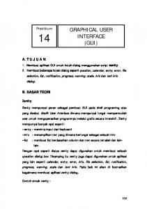
Some of the tools in this category rely on the enrichment of the constraint solver to help improve the visualization, whether by grouping constraints [15] or by keeping explanations of domain reductions [13]. − dynamic visualization and control tools which allow interaction with a CLP process through different visualizations. One example is the Oz-Explorer system [21] where it is possible to jump to any previously encountered state by simply clicking on a node of the search tree, and restart computation from that state. Userguided search is implemented in Oz-Explorer using the first-class computation spaces of Oz. Recomputation is used to trade space for time in Oz-Explorer, and similarly in OPL studio [2], the state restoration mechanisms in tree search are described in [6]. In this paper we propose to push forward these ideas towards a generic architecture allowing the connection of a CLP process to dynamic visualization and control tools. Our ambition is not to realize an ad hoc tool limited to a particular constraint programming system, currently GNU-Prolog [10] and SICStus-Prolog [26], but a generic tool which can be ported to other constraint programming systems as well. One reason for this is that a wide variety of viewers can be useful for debugging or interacting with constraint programs and it is possible in this way to share developments. Another reason comes from the necessity to try different models which often imposes to change of constraint programming systems in order to benefit, for instance, from a particular global constraint. Our approach relies in part on the generic trace format which is defined in the OADymPPaC consortium [19] for post-mortem analysis. We propose to extend this format with a similar generic format for control, and to use these formats for connecting on-line the CLP process to the GUI process. Our current implementation of CLPGUI in Prolog and Java is depicted in Figure 1. Constraint
trace information
Programming System
control
GNU−Prolog or SICStus−Prolog
(XML)
Graphical
Viewers
User Interface
...
Process
Viewers
External viewers
JAVA
Figure 1. Information flow for dynamic visualization in CLPGUI.
Currently, most constraint programming systems do not support however the OADymPPaC trace format and the objective of gener2
icity of CLPGUI with respect to the constraint programming system is therefore quite challenging. The solution used in CLPGUI relies on a non-intrusive tracing and control method based on annotations in the program. Annotation predicates are defined for associating external names to variables, customizing the GUI and more importantly tracing the execution of the program. The originality of this approach lies in the use of annotation predicates not only for sending the specified trace of the execution but also, in the reverse direction, for interpreting control commands, such as recomputing a complete state corresponding to a traced node in the visualized search tree. We show that the annotation predicates form indeed a complete set of control points in the program which can be used to implement in a non-intrusive manner control commands such as backtracking or jumping to a different state represented as a node in the search tree. Besides performance issues which in CLPGUI are largely solved, in order to scale-up, visualization tools have to rely on visualization paradigms that are still effective on large data sets. This difficulty is particularly severe for visualizing very large search trees which is a common need in constraint programming. Apart from [1], the visualization of search trees in three dimensions has not been much investigated. In this paper, we propose a 3D representation of search trees which we found most appropriate to apprehend the shape of large search trees, of 104 nodes for instance. Playing with rotations, that cannot be reproduced in this article, is an important feature of the 3D representation which compensates the compactness of its 2D projection on the screen. Such a robust architecture for visualizing and controling the execution of constraint logic programs can also be exploited to develop application-oriented end-user interfaces in both directions of visualization of solutions and control of the search. We exemplify this aspect of CLPGUI on two placement problems where the user can not only visualize the computed solutions but also modify the constraints or the solutions and search for new solutions near the modified ones. The rest of the paper is organized as follows. Section 2 describes the client-server architecture of CLPGUI and the user console from which the execution of the CLP program can be controlled. Section 3 describes the annotation predicates used for tracing and controlling the execution of the CLP program at various levels of granularity. The interactive execution model of CLPGUI is also described with its implementation in two constraint programming systems: GNU-Prolog and SICStus Prolog with CLP(FD,R) libraries. Section 4.1 presents a dynamic 3D viewer for visualizing the evolution of the domain of variables over time. Section 4.2 describes the representation of the explored search space as partial CSLD derivation trees, and presents different visualizations with 2D 3
and 3D viewers. The following subsection provides some performance figures on a branch and bound optimization problem. Section 5 details the communication mechanism by message passing. Then in Section 6 we show how some application-oriented graphical user-interface have also been successfully developed with CLPGUI on two placement problems, one in virtual reality. Finally, we conclude on the generality of this scheme.
2. Client-Server Architecture
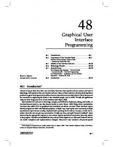
Figure 2. The CLPGUI console.
The graphical user interface of CLPGUI is a Java application connected by sockets as a client to a server which executes CLP goals. Both processes can run on different machines and communicate over the network. This has been experienced with CLPGUI for visualizing the execution of CLP programs on a Workbench of Virtual Reality. The choice of the Java language for implementing the GUI is motivated by several reasons: − its object-orientation, all 3D viewers presented in the following sections inherit from a single class for moving and projecting 3D figures; − the encapsulation of events handling, that is preponderant in dynamic visualization; − the threaded execution, which is mandatory for implementing communication with the CLP process; − its wide availability. 4
For efficiency reasons, we did not use the GL4Java or Java-3D libraries for the generic viewers presented in this paper, as they can directly benefit from ad hoc optimizations that speed-up their incremental display. Nevertheless the architecture can support the use of these powerful libraries for developing complex application-oriented viewers, as shown in section 6.2. During initialization, the CLP server starts an interpreter of the command lines received on the socket. The GUI Java client opens a graphical console such as the one in Figure 2. That console is used for establishing a connection to the CLP server, and for posting constraints or executing arbitrary CLP goals. The CLP program may contain annotations for creating buttons for some constraints or for some Prolog goals to execute in an interactive manner. These buttons for posting constraints or Prolog goals then appear at the bottom in the CLPGUI console, see Figure 2. Since these buttons rely on the annotation predicates discussed in the next section, they are completely independent of the underlying constraint system. A click on the button posts the constraint or executes the goal associated to the button. Other arbitrary goals can be executed by entering them in a text field. In addition, one button called “backtrack” continues the execution of the current goal up to the next success, or, if there is no more success, returns to the state of the previous interaction. Another button called “backtrack to last interaction” forces backtracking to the state of the previous interaction. The menu bar of this console contains menus to select and activate the viewers of the search tree or of the finite domain variables. 3. Non-Intrusive Traces and Control through Annotations Annotations have been proposed as a simple mechanism for tracing the execution of constraint logic programs and specifying the level of granularity of the data to visualize [5]. In this section, we present the main annotation predicates defined in CLPGUI and we show how annotation predicates can be extended to an active mechanism for interpreting control commands as well in a non-intrusive manner. 3.1. Annotation Predicates In CLPGUI, the CLP program may contain annotations for giving an external name to CLP(FD) variables, for creating buttons for posting constraints or goals from the CLPGUI console, and for specifying the goals to visualize in the search tree. The following predicates are part of the annotation library: 5
− gui varnames(LV,LN) and gui varnames(LV) give an external name to the list LV of CLP variables. These external names are used in the graphical user interface and for the communication by sockets. If no names are provided, standard names V1, V2, . . . are created. − gui button(goal) creates a button in the GUI console for executing a goal or for posting a constraint. − gui bagof buttons(goal, call) creates a bag of buttons for each successful instance of the second argument. − gui trace search(goal) executes the goal and traces the execution of that goal, by creating nodes in the search tree. The goals and constraints posted from the graphical console are always traced. − gui show domains updates the visualization of the current state of FD variables. The advantages of annotations are: − the flexibility of defining different levels of granularity concerning the information to visualize, − the easiness for making existing programs interactive, − the portability of the GUI to other constraint programming systems, as all communications with the GUI are encapsulated in the implementation of annotation predicates. The limitations of annotations are well-known in standard programming environments: they may be difficult to maintain in large programs. In that case, one solution is to automatically generate annotations with a graphical editor of the program source, where spy points and trace options can be specified. Nevertheless, one peculiarity of constraint logic programming is the conciseness of programs. CLP(FD) programs for solving combinatorial optimization problems on real-size data may compute with a huge amount of constraints and variables, but the program source for handling constraints and defining complex search strategies usually remains relatively concise. Therefore in this context, the proposed annotations appear as a satisfactory solution. In many CLP systems however, the heuristic labeling procedures are built-in, and may be difficult to trace precisely with simple annotations. This is possible if the CLP system provides coroutining facilities like for instance the freeze predicate) of SICStus-Prolog [26]. In this case, 6
one can trace the instantiation of variables and the search tree created by the built-in labeling procedure, with a simple call to the following predicate before labeling: freeze_trace([]). freeze_trace([X|L]):- freeze(X,gui_trace_call(X=X)), freeze_trace(L). In absence of coroutining predicate, one solution is to rely on the tracing facilities of the CLP system in order to extract, and communicate to the GUI, the relevant information, like the creation of a choice point or the reduction of one variable’s domain. Another solution is to program the labeling heuristics in the host language, in order to make available the information coming from the constraint solvers that is relevant to the search heuristics. In that case, the effect of the search strategy can be visualized at different levels of granularity. In its simplest form, a predicate for tracing a labeling procedure can be defined with a gui trace search annotation as follows: gui_trace_labeling([]). gui_trace_labeling([X|L]):- gui_trace_labeling(L), gui_trace_search(fd_labeling(X)). It is worth noting that if the search strategy is implemented with a meta-interpreter, and uses constraint posting instead of labeling (like in the bridge problem described in section 4.3), the relevant part of the search tree can always be traced with CLPGUI annotations. A similar difficulty arises for tracing internal constraint propagation steps. This is not possible without access to the wakening events of the constraint solver, as defined for instance in the OADymPPaC format [19]. The annotations for tracing constraint propagation steps have thus to rely either on coroutines or on the tracing facilities of the solver in order to extract and communicate constraint wakening events. An XML syntax for traces has been defined by the OADymPPaC consortium for this purpose. Example 1. The following annotated GNU-Prolog program solves the well known SEND+MORE=MONEY puzzle in an interactive manner, by creating buttons for posting the constraints and for trying two labeling goals in this example: sendmore(L):L=[S,E,N,D,M,O,R,Y], gui_varnames(L,[’S’,’E’,’N’,’D’,’M’,’O’,’R’,’Y’]), fd_domain(L,0,9), gui_show_values, 7
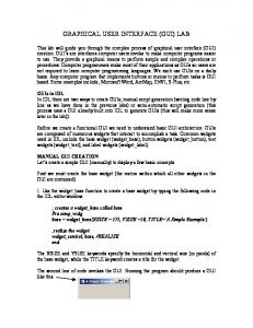
gui_button(fd_domain([S,M],1,9)), gui_button(1000*S+100*E+10*N+D+1000*M+100*O+10*R+E #= 10000*M+1000*O+100*N+10*E+Y), gui_button(fd_all_different(L)), gui_button(gui_trace_labeling(L)), reverse(L,L2), gui_button(gui_trace_labeling(L2)). This program generates the console in Figure 2. The evolution of the finite domain variables over time, after the posting of constraints and of the first labeling goal, is depicted in Figure 5. The visualization of the search tree for obtaining all solutions under the first labeling goal, and then under the second labeling goal executed after a backtracking command, is depicted in Figure 3. Under the first ordering, the labeling is deterministic. Under the second ordering, few backtracking steps occur on variable Y when searching for other solutions. Note that other labeling heuristics can be tried directly from the console. On such pedagogical examples, the advantage of immediately visualizing the effect of posting a constraint or trying a labeling, is clear for teaching purposes, since the user can see at the same time the number of backtracks, the depth of the search, and the evolution of the domains of the variables.
Figure 3. Search trees SEND+MORE=MONEY.
with
two
labeling
orderings
in
the
puzzle
Example 2. The following program solves the N queens problem by creating buttons for posting the constraints (safe predicate) and labeling goals for each variable (fd labeling predicate) and for all variables (gui trace labeling predicate). queens(N,L):8
length(L,N), fd_domain(L,1,N), gui_show_values, gui_button(safe(L)), gui_bagof_buttons(fd_labeling(X),member(X,L)), gui_button(gui_trace_labeling(L)). Three visualizations of the search tree for one single execution of the above program for the 8 queens problem are depicted in Figures 6, 7 and 8. 3.2. Control through Annotations Annotations in the program provide a set of control points which can also be used to implement a sophisticated control of the execution of the constraint program in a non-intrusive manner. In CLPGUI we use annotation predicates to implement the automatic recomputation of any state represented as a node in the search tree. Once a node in the search tree (such as the tree depicted in Figure 3) has been selected for being recomputed (by clicking on it), a recomputation directive is transmitted to the solver by means of the path in the tree from the root to the node. This path is then interpreted as a sequence of choices that have to be taken from the initial state to the one being recomputed. The algorithm is thus basically the classical recomputation algorithm of a path in a derivation tree [21, 2, 6], where actually no intermediate state is memorized. The novelty in CLPGUI is that this recomputation algorithm is implemented in a non-intrusive manner using annotation predicates to control the execution of the CLP process following the recomputation path. This recomputation algorithm supports CLP programs containing cuts and exceptions. It does not support however programs containing side effects. One way to support side effects would be to recompute not only the path but the entire derivation tree leading to the recomputed node. Another way would be to memorize the intermediate state values that are subject to change by side effects. A particular case of this is the memorization of the best cost value in optimization predicates, such as in the CLP predicate minimize(Goal,Cost) for instance. Batch recomputation, i.e. memorizing all constraints posted in a node and adding all constraints at once for a recomputation, has been proposed in [6] as a method giving slightly better performances. It is worth noting however that this method is not applicable in our non-intrusive setting as we do not assume a complete knowledge of all constraints posted by the program. 9
3.3. Interactive Execution Model for CLP The interactive execution model of the CLP process used in CLPGUI is a combination of the model for adding and removing constraints and goals described in [12] with the non-intrusive recomputation algorithm described above. In CLPGUI, constraints and goals can only be added to the current goal; the removing of constraints or goals occurs by backtracking or jumping to a specific node. It is therefore possible on a success of the current goal: − to add constraints or any goals to the current goal and continue resolution, − to backtrack to the next success (command “backtrack” of Section 2), − to backtrack to the previous interaction (command “backtrack to last interaction”), − or to recompute a given state depicted as a node of the search tree. It is worth noting that such a top level is in fact very appropriate for standard Prolog systems. Our current implementation uses the global variables of GNU-Prolog [10] to memorize global information, such as input and output sockets, variable names, and information used for backtracking. Global variables make it possible to avoid adding parameters to many predicates and lead to a simple implementation of annotations. In SICStus-Prolog [26], global variables are emulated using blackboard predicates, mutables and system predicates.
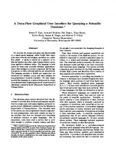
4. Generic Viewers for Debugging or Teaching 4.1. 2D and 3D Views of Finite Domain Variables The domains of finite domain variables at any given time can be visualized with a generic 2D boolean matrix having one row per variable and one column per value. In the N-queens problem this view provides a view of the chessboard. In a scheduling problem, like the famous bridge problem [27], this view shows the possible starting dates of the task and the flexibility of a solution, as depicted in Figure 4. The evolution of finite domain variables over time can be visualized in a three dimensional graph variable-domain-time, as already proposed in the VIFID/TRIFID tool [25]. In CLPGUI the visualization is dynamic, the Java process reads the stream of finite domains information 10
Figure 4. 2D view of finite domain variables in an optimal solution of the bridge scheduling problem [27].
and paints the figure in an incremental manner. Domains are depicted by their size on the vertical axis, see Figure 5. According to options, that can be set in the CLP program or in the GUI, only the size, the interval or the complete domain of variables is visualized. But in any case only the sizes of the domains are memorized, therefore the extra information is lost when the figure is repainted. The time axis traces the interactions (i.e. the posting of constraints in the example), and the execution of traced goals (i.e. the labeling in the example). This view shows that the posting of constraints instantiate variables S, M, O and that the first labeling step on variable E in fact instantiates all variables by constraint propagation. An option determines whether backtracked states are traced or erased. The figure can be moved, zoomed and rotated. For efficiency reasons, the rotations are limited to a quadrant of a sphere which is not a real limitation for the user. In this way the visible faces are efficiently determined and the figure can be drawn incrementally. Extra information on variables and executed goals can be obtained by moving the mouse over the position of a variable or on a time position. The 3D dynamic view of finite domain variables evolution is very useful for teaching constraint programming. The effect of constraints 11
Figure 5. Dynamic 3D view SEND+MORE=MONEY.
of
finite
domain
variables
in
the
puzzle
is immediately seen and many strategies can be tried step by step. The possibility for a student to see the domain reductions as they are happening is really helpful for understanding the underlying machinery of constraint programming. On larger sets of variables, the 3D view of domains can still be useful to get a view of the pruning power of different constraint models, and of the efficiency of different search heuristics, by comparing the general shape of domain reductions. 4.2. 2D and 3D Views of the Search Tree 4.2.1. Partial CSLD derivation trees The search tree considered in CLPGUI is a labeled tree defined as follows: − a node is introduced for each call to a traced goal (called a call node), and for each success to a traced goal (called a success node), − the label of a call node is the called goal, − the label of a success node is the list of named variables with their value, − the arcs correspond to the operational CLP transitions. 12
Figure 6. 2D view of the search tree in the 8-queens problem.
This tree, which is a subtree of the CSLD derivation tree [17], is a quite natural representation of the search tree for describing CLP program execution. A branch represents a conjunction, and the different successors of a node represents a disjunction. A success node may have several successors if there is an untraced non-deterministic goal which is executed after the success, and before the next call to a traced goal. This is the main reason why success nodes are introduced in partial CSLD trees. In this way, the non-determinism due to untraced goals cannot be confused with the non-determinism of traced goals. One disadvantage of CSLD trees is that when dealing with deterministic programs they are threadlike and thus space consuming in their standard representation. AND-OR trees provide a more compact representation, as the threadlike parts of the CSLD tree are compacted in the successors of a single AND-node. For this reason, in the context of logic programs where most predicates are deterministic, AND-OR trees, and their variant AORTA diagrams which indicate the status of resolution of the goals, have been preferred [11]. Nevertheless in the context of constraint logic programming over finite domains, the situation is quite different. The search tree to visualize is usually focused on the labeling predicates, or more generally on the branching procedure, which is highly non-deterministic (at least during debugging). The representation of the deterministic part of the search tree with threadlike 13
Figure 7. 3D of the search tree in the 8-queens problem.
structures provides an immediate visualization of the pruning power of constraints. A naive solution for tracing constraint propagation steps in this approach is to add deterministic nodes for tracing constraint wakening events. For space limitation reasons, it is preferable however to aggregate constraint propagation information to the nodes of the search tree. This is proposed in the “Christmas trees” of OPL studio [2]. For search engines not based on backtracking, it is worth noting that a partial CSLD derivation tree can still provide a valid representation of the explored search space, as long as the explored states can be defined by their relation to some ancestor states. A formalization of an interactive constraint solver by transformations of CSLD derivation trees was done in [12]. 4.2.2. Search Tree Viewers Once the search tree is formally defined, it can still be visualized in many ways, and in some cases it can be interesting to use several visualizations at the same time. We have currently implemented several two-dimensional and three-dimensional viewers, but many more representations could be imagined and fruitfully used. In all the following representations, the labels of the nodes are visualized when the mouse is moved over them, and there exists an option 14
Figure 8. Dual treemap representation obtained by rotation of the 3D view.
for making all nodes visible. The successes are materialized by a red cross. Each view can be moved, zoomed and rotated. Figure 3 uses a standard 2D representation of the search tree in a fixed width. Figure 6 uses a dynamic 2D representation of the tree with a fixed spacing between leaves. This representation of the tree can be drawn incrementally and is thus appropriate for the dynamic visualization of large trees. To our knowledge, the 3D visualization of search trees has not been much investigated. Figure 7 shows a somewhat original 3D representation of the search tree with alternating planes of successors. One advantage of this 3D representation is that it is relatively compact, it helps visualizing rather large trees by playing with rotations, see Figure 11 for another example. Our experience is that the 3D view is the most appropriate view to apprehend the shape of large search trees. It is interesting to note that one obtains a dual treemap representation of the tree by rotation of the 3D alternate tree up to its vertical projection, as done in Figure 8. Treemap representations (with colors for aggregating information) are known to be particularly efficient for representing large data sets [20] and for visualizing complex phenomenons such as correlations, patterns or symmetries. By rotating the 3D tree up to its vertical projection, one obtains a dual view of the treemap where the centers of the rectangles instead of the rectangles 15
Figure 9. Complete search trees for all solutions to the 8 queens problem, without and with symmetry breaking obtained by adding the constraint V0#