Cluster-based Routing Overhead in Networks with ... - RPI ECSE

Cluster-based Routing Overhead in Networks with Unreliable Nodes Huaming Wu and Alhussein A. Abouzeid Department of Electrical, Computer and Systems Engineering Rensselaer Polytechnic Institute, Troy, New York 12180 Email: [email protected], [email protected]

Abstract— While several cluster based routing algorithms have been proposed for ad hoc networks, there is a lack of formal mathematical analysis of these algorithms. Specifically, there is no published investigation of the relation between routing overhead on one hand and route request pattern (traffic) on the other. This paper provides a mathematical framework for quantifying the overhead of a cluster-based routing protocol. We explicitly model the application-level traffic in terms of the statistical description of the number of hops between a source and a destination. The network topology is modelled by a regular two-dimensional grid of unreliable nodes, and expressions for various components of the routing overhead are derived. The results show that clustering does not change the traffic requirement for infinite scalability compared to flat protocols, but reduces the overhead by a factor of O(1/M ) where M is the cluster size. The analytic results are validated against simulations of random network topologies running a well known (D-hop Max-min) clustering algorithm.

I. I NTRODUCTION Ad hoc networks are comprised of nodes that perform multi hop packet forwarding over wireless links. The routing protocols for ad hoc networks can be divided into two categories based on when and how the routes are discovered: proactive and reactive. In proactive routing protocols, consistent and up-to-date routing information to all nodes is maintained at each node, whereas in reactive routing the routes are created only when needed. In this paper, we focus on reactive routing protocols. To support large scale ad hoc networks, numerous clusterbased routing algorithms have been proposed [1], [2]. In cluster-based routing, the network is dynamically organized into partitions called clusters with the objective of maintaining a relatively stable effective topology. The membership in each cluster changes over time in response to node mobility, node failure or new node arrival. Clustering techniques are expected to achieve better scalability since most of the topology changes within a cluster are hidden from the rest of the network. However, clustering incurs a cluster maintenance overhead, which is the amount of control packets needed to maintain the cluster membership information. In hierarchical routing protocols, intra-cluster (inter-cluster) routing refers to the routing algorithm used to find a route between a source and destination within the same (belonging to different) clusters. Typically, inter-cluster routing is reactive while intra-cluster routing is proactive. In this paper, we develop an analytical model that captures the essential characteristics of cluster-based routing

algorithms. The algorithm considered in this paper employs reactive routing for inter-cluster routing. Within each cluster, the cluster-head proactively maintains paths to all member nodes. We model the network topology by a two dimensional regular degree-4 grid. We focus on situations where topology changes because of node failure rather than node movement. Such situations are commonplace in many sensor network applications where cluster-based routing is suggested [3]. Our objective is to mathematically characterize the scalability properties of these protocols under different traffic patterns. In this paper, the term ‘traffic’ refers to routing-layer traffic, which is the pattern of route (i.e. path) requests. The traffic model is described in Section II. We primarily focus on routing overhead as a measure of scalability. We define the routing overhead as the average amount of routing protocol control packets in the network. Analytic expressions of the different types of control packets are derived. These expressions provide insights into the impact of the communication traffic patterns on the performance of routing protocols. Our previous work [4] considered flat routing protocols only. In this paper, we investigate the impact of clustering on the scalability of routing protocols. It is important to note that this work does not attempt to model or compare between specific details of cluster-based routing protocols - rather, to capture the essential characteristics and scalability limits of this class of protocols by deriving lower bounds on the overhead. Up to our knowledge, only [5] and [6] attempt to analytically quantify routing protocols control packet overhead in ad hoc networks. In [6], overhead of Hierarchical Link State (HierLS) routing protocol is considered. In [5], overhead required for constructing and maintenance of routing tables in a hierarchically organized network is considered. However, both analysis were performed to primarily address the overhead of cluster formation and maintenance incurred by node mobility, and they do not consider the effect of the route-request pattern on the scalability of routing protocols. The remainder of this paper is organized as follows. The network model is presented in Section II. Section III provides a detailed analysis of routing overhead of a generic cluster-based protocol. Section IV checks the validity of our analyticallyderived conclusions by conducting simulations of a specific implementation of hierarchical routing algorithm in random

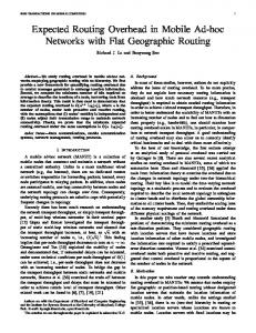
network topologies. Finally, we summarize the main results of the paper and outline possible avenues of future work in Section V. II. N ETWORK M ODEL As mentioned earlier, this work doesn’t attempt to model the specific details of cluster-based routing protocols - rather, to capture the essential characteristics and scalability limits of this class of protocols by deriving lower bounds on the overhead. To achieve this, we present in this section a description of a generic cluster-based routing protocol. Since we are interested in modelling a network with node failures, we assume that nodes fail (or more precisely, turned to “OFF” state) randomly. However, nodes are assumed to return back to operation (i.e. “ON” state) quickly, such that on the average, most nodes are turned ON most of the time. In other words, we are interested in modelling the overheads in maintenance due to node failure, but we assume during our analysis that given a node failure, all other nodes have not failed. This necessitates this assumption. This is true if the probability that a node turns off is much less than the probability that a node turns on. A. Topology Model We assume an infinite number of nodes is located at the intersections of a regular grid. Two hosts within range of each other can communicate, and are said to be neighbors. The transmission range of each node is limited such that a node can directly communicate with its four immediate neighbors only. For example, in Figure 1, node 1 can directly communicate with nodes 2, 3, 4 and 5. Figure 1 illustrates the a clustered hierarchy. The cluster head is assumed at the center of a cluster. Red (darkest) nodes are cluster heads. White nodes are gateways for adjacent clusters. For simplicity, we assume clusters have equal size. The cluster radius M is the distance from a cluster head to a gateway node. We assume that all the nodes use a common wireless channel for communication. Medium Access Control (MAC) layer collisions are neglected in the analysis. B. Model of Routing Layer Traffic From a routing protocol perspective, ‘traffic’ could be defined as the pattern by which source-destination pairs are chosen. In previous simulation studies of routing protocols, source-destination pairs are usually chosen according to a uniform distribution (e.g. [7]). In this paper, we propose a more general traffic pattern in which the choice of a sourcedestination pair could depend on the distance (in terms of number of hops along the shortest path) between them. Let (xi , yi ) denote the coordinations of node i. Define the distance between two nodes i and j as: ri,j = |xi − xj | + |yi − yj | . In the following, all distances between nodes are counted in number of hops. The probability that two nodes are an active source-destination pair is assumed to decrease with the distance between the two nodes. More specifically,

5

2 1

3

4

Fig. 1. Hierarchical grid network. Red (darkest) nodes are the cluster heads. For example, nodes located in a dashed rectangle are organized into a cluster with radius M = 2. Clusters communicate via gateways (white nodes).

k pi,j = c/ri,j , where c is a constant. Because of the symmetry, it will be more convenient to drop the subscripts from the above equation when it is understood and use p(r) instead. Thus, c p(r) = k (1) r where r is the distance between the node initiating the new path request and the destination node. We can control the traffic pattern by changing k. The communication sessions are independent of each other.

C. Hierarchical Routing Protocol Model We consider a generic cluster-based routing protocol. Although details of clustering algorithms clearly depend on the specific protocols, we try to identify some common principles that can be applied to various reactive cluster-based routing protocols [1], [8]. Routing overhead can be attributed to one of the following events: • new session arrival; • node failure on the active path; • cluster maintenance due to node failure. and thus only relevant routing protocol behaviors are described below. 1) Clustering: Clustering is a method by which nodes are placed into groups, called clusters. A cluster head is elected for each cluster. A cluster head maintains a list of the nodes belonging to the same cluster. It also maintains a path to each of these nodes. The path is updated in a proactive manner. Similarly, a cluster head maintains a list of the gateways to the neighboring clusters. When a node changes its state from OFF to ON, it sends out a message requesting to join a cluster. Its neighbors hear this

“join” message and at least one of them reports to the cluster head. Then this cluster head records the newly joined node into its member list, computes a path to this new node and sends back an “accept” message which contains the identity of the cluster-head and the new path. Thus, every member node knows its cluster head and a path from itself to the cluster head. When a member node fails, at least one of its neighbors reports this node failure to the cluster head. If a cluster head fails, this cluster has to be re-organized. 2) Route Discovery: Route discovery is the mechanism whereby a node i wishing to send a packet to a destination j obtains a route to j. When source node i wants to send a packet to destination node j, it first sends a Route Request (RREQ) packet to its cluster head along the shortest path. There are two cases. If j is within the same cluster of i, cluster head of i sends the route information to i immediately. In reactive routing protocols, i finds a route to j by flooding. Otherwise this cluster head will flood the network by a RREQ packet at the cluster head level (i.e. through gateways of clusters). Each RREQ packet is initialized with some value called Time to Live (TTL) in the header of the packet. When forwarding an RREQ packet, each node decrements the TTL upon each transmission (such as limited broadcast in [9]). If the initial TTL value is large enough, an RREQ packet arrives to j’s cluster head (we assume the network is connected). j’s cluster head then sends out a Route Reply packet (RREP). The RREP packet travels across the shortest path 1 back to the cluster head that initiated the RREQ flooding. Finally, i will receive a Route Reply (RREP) from its cluster head which contains a source route to j. 3) Route Maintenance: Route maintenance is the mechanism by which a node i is notified that a link along an active path has broken such that it can no longer reach the destination node j through that route. When route maintenance indicates a link is broken, i may invoke route discovery again to find a new route for subsequent packets to j. In reactive protocols, route maintenance for this route is necessary only when i is actually sending packets to j. We consider a source-route based reactive routing algorithm (as in [1]). In flat routing protocols like [10], if a node fails, the links associated with this node are broken. Then, neighboring nodes of the failed node detect the broken links and send a Route Error (RERR) message to each source node that has sent a packet routed through the broken links. Each RERR message will travel along the reverse route from the node reporting link breakage to the source node. In cluster-based routing, the neighboring node sends an RERR packet to its cluster-head (rather than the source node). The cluster-head could ‘patch’ a path locally without informing the source node (using the topology information stored at the cluster-head) if the failed node is not the destination node. 1 While forwarding the RREP, each intermediate cluster head will calculate an optimized hop-by-hop route within its cluster using its stored topology information about its own cluster. Thus, node i gets a shortest path route to node j.

This is called local repair [1]. In this case, the path is locally fixed. Otherwise, the RERR packet is forwarded to the source node. III. A NALYSIS The overhead of cluster based routing can be associated with one of the following operations: Route Discovery, Route Maintenance and Cluster Maintenance. Prior to deriving expressions for the routing overhead, we establish some notations and derive some preliminary results. We use the same notations as in [4]. We will refer frequently ∞ P to the following summation: f (k) = 1/rk , where k > 1 r=1

is required for the convergence of this summation. M denotes the radius of a cluster (defined earlier in this paper). • D(r): the number of nodes located at a distance r away from a node. D(r) = 4r (2) •

N (r): the number of nodes located within a distance r from a given node. N (r) = 2(r2 + r)

•

pR (r): the probability that two nodes a distance r apart are an active source-destination pair. pR (r) =

•

(3)

1 r k−1

f (k − 1)

;k > 2

(4)

Z is a random variable that denotes the number of hops that an active session travels. E[Z] denotes the expected value of Z. f (k − 2) E[Z] = ;k > 3 (5) f (k − 1)

The derivations of the above four expressions are included in [4]. • Nf ind denotes the total number of RREQ packets per new route discovery. Every transmission of the same packet is counted as a separate transmission. E[Nf ind ] denotes the expected number. • Nof f denotes the total number of route error packets needed to notify others about a node failure. E[Nof f ] denotes the expected number. • Nclus denotes the total number of control packets needed to maintain a cluster if a node fails within that cluster. E[Nclus ] denotes the expected number. There are two levels of hierarchy; level-0 which refers to the flat network topology (i.e. topology formed by the nodes of the network) and level-1 which refers to a virtual topology in which each node is a cluster. Similarly, we define two kinds of distance, level-0 distance (or hop distance) which is the number of hops between two nodes at level-0 and level-1 (or cluster distance) which is the number of hops between two nodes at level-1. Lemma 3.1: A hop distance r between two cluster-heads (at r the level-0 topology) is mapped into a cluster distance l = 2M (at the level-1 topology). At the level-1 topology, the number

of nodes (i.e. clusters) located at a cluster distance l from a particular cluster is Dc (l) = 4l (6) Proof: From Figure 1, we can see that cluster heads organize into a level-1 network with hop distance 2M between adjacent cluster heads. Let O denote a particular cluster head. For any given positive integer l, there are a total of l + 1 clusters at a cluster distance l from cluster head O located in each of the four quadrants (Figure 1). Summing over the four quadrants yields 4(l + 1). Removing the four double counted clusters, the total number of clusters is 4l. From the above result, we can easily deduce the following result. Corollary 3.2: The total number of clusters which are within a cluster distance l from a given cluster is: Nc (l) = 2(l2 + l)

d1 d2

d12

d3

d11

h s

d4

d10

d5

d9 d8

d6

(7)

d7

A. Route Discovery From our routing protocol model in section II-C.2, route discovery involves an RREQ and an RREP process. The overhead for RREQ is generally higher than the RREP since it may involve flooding at the cluster head level. Hence, we focus our analysis on the RREQ overhead. In the following derivation, we assume that in the case of cluster-level flooding of an RREQ packet, the TTL field will be set equal to the minimum TTL value needed to reach the destination cluster. This assumption results in a lower bound for the route discovery overhead since practically the TTL field is not known a-priori. Hence actual protocol implementations either (a) use a higher value of the TTL which results in higher overhead or (b) use an expanding ring search [11] which still incurs higher overhead. Theorem 3.3: Considering a source node at distance j hops from its cluster head, the number of RREQ packets Nf ind (r, j) required to find a destination that is a distance r from the source node obeys j + 4M ∗ (n2 + n) ≤ Nf ind (r, j) ≤ j + 4M ∗ (n2 + n) (8) where n = round(|r − j|/2M ), n = round((r + j)/2M ). round(x) is the nearest integer of x. Proof: Assume that the source node s is j hops away from its cluster head h. The distance y from destination to the source cluster head is of interest since the level-1 flooding of RREQ is initiated from the head h. y depends r, j and the positions (xs , ys ), (xh , yh ) and (xd , yd ) of the three nodes. For example, in Figure 2, j = 2 and r = 3, but y is different for different destination nodes d1 ∼ d12 . However, there are always two extreme cases for every source node: the best case with ymin = |r − j| and the worst case with ymax = r + j. Thus, the flooding of RREQ packets initiated by node h must cover at least 2M ∗ round(|r − j|/2M ) hops and at most 2M ∗round((r +j)/2M ) hops to reach the destination cluster head. Since the hop distance between neighboring clusters is 2M , the total RREQ packet retransmissions is the same as the number of clusters within a circle centered at source cluster

Fig. 2. Route discovery example. s is the source node which is j = 2 hops away from its cluster head h. There are 12 destinations d1 ∼ d12 all at r = 3 hops away from s.

head h. From Lemma 3.1, for any cluster distance n ∈ [n, n], Nf ind (r, j) = j + 2M

n P

4l = j + 4M (n2 + n)

l=0

Theorem 3.4: Considering the best case for every source node, the minimum average overhead of finding a new route E[Nf ind ]min is f (k−3)(6M +6+3/M )+f (k−2)(4M 2 +2)−f (k−1)M (M 2 −1) 3(2M 2 +2M +1)f (k−1) Proof: Let nj denote round( |r−j| 2M ). We notice that

(9)

|r − j| j−r ) = round( )=0 2M 2M when r < j since r ≥ 1 and 1 ≤ j ≤ M . Thus in the following, we only need to consider r ≥ j. Also, because r and j are independent of each other. The minimum average of Nf ind (r) is nj = round(

E[Nf ind |r]min = r 2 r 4M [ 2M + 2M ]+

M P

M P

+

j=1

4j [j + 4M (n2j + nj )] N (M )+1

2

r−j 4j[j+4M { r−j 2M + 2M }]

j=1 2M 2 +2M +1 2

≈ =

4M (n20 +n0 ) N (M )+1

2

2

(round( r−j 2M ) ≈

r (2M +2+1/M )+r(4M /3+2/3)−M (M −1)/3 2M 2 +2M +1

Then the minimum average of Nf ind is ∞ P E[Nf ind ]min = pR (r)E[Nf ind |r]min r=1 ∞ P 2M +2+1/M 4M 2 /3+2/3 M (M 2 −1)/3 r k−3

+

r k−2

−

r k−1

=

r=1

=

f (k−3)(6M +6+3/M )+f (k−2)(4M 2 +2)−f (k−1)M (M 2 −1) 3(2M 2 +2M +1)f (k−1)

(2M 2 +2M +1)f (k−1)

r−j 2M )

B. Route Maintenance We make the optimistic assumption that local repair will succeed for all active paths except for those terminating at the failed node. Also, the RERR packet sent from a neighboring node of a failed node to the cluster head is considered as Cluster Maintenance overhead in Section III-C. In this case, an RERR packet will be sent to the source of each active session that ends at the failed node from neighboring nodes of that failed node, independently (i.e. even if some of the sessions might have portion of the routes are common). Theorem 3.5: E[Nof f ] = 4c(f (k − 2) − f (k − 1)); k > 3 (10) Proof: Let o denote the failed node in the network, and let r denote the distance from a source node s to the destination node o. Following the assumption that nodes always communicate along shortest paths, there are (r − 1) hops from neighboring node of o to the source node s. There are total 4r nodes a distance r away from node o. The average number of RERR packets is E[Nof f ] =

∞ P

(r − 1)4rp(r) = 4c

r=1

∞ P r=1

= 4c(f (k − 2) − f (k − 1))

1 ( rk−2 −

1 ) r k−1

C. Cluster Maintenance We consider the overhead of cluster maintenance incurred by a node failure. There are two cases: (a) If a cluster head fails, only this cluster has to be re-organized. This procedure does depend on the clustering algorithm. Based on the analysis of [12], formation of Dhop clusters requires 2D runs of flooding over a cluster. The theoretical minimum number of routing packets to re-organize a cluster due to the cluster head failure is 2M ∗ (N (M ) + 1) in a cluster with radius M . (b) If a member node fails, the neighbors detect link failure and at least one neighboring node informs the cluster head. Assume r is the hop distance from the failed node to its cluster head. Then it takes r − 1 hops to reach the cluster head. Combining the two cases above yields following expression for the average cluster maintenance overhead. Theorem 3.6: M P ∗(N (M )+1) + 4r ∗ (r − 1) N (M1 )+1 E[Nclus ] = 2MN (M )+1 =

4(M −1)M (M +1) 3(2M 2 +2M +1)

r=1

+ 2M (11)

D. Scalability of the Hierarchical grid From the previous results (9), the minimum average routing overhead for a node is bounded for an infinite grid if the coefficient k is larger than 4. Thus, compared with the scalability results of flat routing protocols in [4], the introduction of 1-level hierarchy does not change the traffic condition required for infinite networks scalability. However, the overhead of route discovery decreases by a factor of

O(1/M ) of flat routing protocols overhead [4]. The average number of RERR packets is bounded for an infinite grid if k > 3 and is independent of the cluster size. The cluster maintenance overhead due to node failure is in the order of O(M ). Therefore ,we have the following result. Corollary 3.7: The hierarchical grid becomes infinitely scalable only if the coefficient k is larger than 4. This result, among others, is validated in the following section. IV. N UMERICAL R ESULTS AND S IMULATIONS To verify our analysis, we build a simulator by MATLAB. We use D-hop Max-min clustering 2 algorithm [12] in our simulations. N nodes are randomly distributed over a square area of side length L. Though our analysis is based on a regular grid, we run simulations for random network topologies in order to check the validity of the analysis regarding the scalability as a function of k for a wider set of topologies. Since it is impossible to simulate an infinite grid, an issue arises in how to compare the analytical results with simulations. We replace the upper limit in each summation in our results by the proper value that depends on the size of the finite grid used in simulations. However, this doesn’t take care of the edge effects that will arise in the simulations, which causes deviations from the analytical results. We consider five networks of size N = 100, 225, 400, 625 and 1225. Let r0 denote the communication radius of a node, which is the same for all the nodes in the network. Let g denote the average number of nodes within a direct communicate area of a given node (i.e. average degree of a node). From [13], the average node degree should be O(log N ) to keep the network asymptotically connected. We choose g = 15 and r0 = 20 in our simulations. The sideplength L of every network size is calculated from L = r0 N π/g. For every network size, a fully connected topology is generated (we generate a number of topologies, check the connectivity of each using standard methods, and select only those that are connected). Then for every topology, we run Floyd-Warshall [14] algorithm to get the connectivity matrix whose elements indicate the number of hops between each node. As the goal of our simulation is to verify our analytical results, other traffic characteristics such as time duration are irrelevant. The sourcedestination pairs are chosen according to (1) where the hop numbers between each node are obtained from the connectivity matrix. Each data point represents an average of at least five runs with identical topology, but different source-destination patterns. We ran simulations after all nodes organized into clusters. To study the impacts of k and M on the route discovery overhead, we set up the following simulation scenarios. For each node, we initiate communicating sessions from that node. For every session, we measure the number of RREQ packets (source node to cluster head and flooding at cluster head level if needed). Shortest path routing is assumed here as in 2 We don’t use CBRP [1] since the cluster head only has 2-hop topology information.

5.5

4.5 4

Average number of RERR packets per node failure

5

Average number of RREQ packets per node

14

M=3,k=4 M=3,Theory,k=4 M=3,k=4.5 M=3,Theory,k=4.5 M=6,k=4 M=6,Theory,k=4 M=6,k=4.5 M=6,Theory,k=4.5

3.5 3 2.5 2 1.5 1 0.5 0

0

200

400

600

800

1000

1200

1400

Total number of nodes

k=3 Theory, k=3 k=3.5 Theory, k=3.5

12

10

8

6

4

2

0

0

200

400

600

800

1000

1200

1400

Total number of nodes

Fig. 3. Minimum average number of RREQ packets per source node E[Nf ind ]min , c = 0.1. Theoretical results calculated according to (9). k > 4 for convergence.

Fig. 4. Average number of route error packets per destination node E[Nof f ], c = 0.5, M = 3. Theoretical results calculated according to (10). k > 3 for convergence.

our analysis. Then we count the average number of RREQ packets for a source node, which is shown in Figure 3. In the simulation scenarios with M = 3 or 6, we observe that the average number of RREQ packets continues increasing as the size of the network increases when k = 4. But when k = 4.5, the average number of packets increases for small network size, and then becomes flat for large network sizes. All the simulation results have the same trend as theoretical results. The second experiment verifies the results of Theorem 3.5. The theory results are according to (10). For the simulations of route error notification, we set up communicating sessions for each node. After every session has run for a long time (enough for every source node to find a route to destination) to avoid transient effects, the destination node is turned off. Then we count every route error packet sent from neighboring nodes of the failed node. Clearly, notification of route error due to node failure only depends on traffic pattern. The simulated results for M = 3 are plotted in Figure 4. Note that the theoretical results may not be always less than the simulation results since, unlike the route discovery overhead, our expression for the route maintenance overhead is not a lower bound.

routing protocol. Further, only a two-level hierarchical grid is considered. The effect of multilevel clustering is left for future work.

V. C ONCLUSION In this paper, we developed a mathematical analysis of the overhead of a cluster-based routing protocol in an unreliable network. The protocol performance in terms of route discovery, route maintenance and cluster maintenance is investigated. According to our model, although cluster-based routing may decrease routing overhead, it does not change the traffic requirement for infinite scalability compared to flat routing protocols. Our analytical results point to the key role that the traffic pattern plays in defining the scalability of these protocols. Expressions for various quantities of interest, as well as conditions for scalability were derived and validated via simulations. Several avenues of future work remains, including the analysis of the impact of MAC layer interactions with the

R EFERENCES [1] Y. T. Mingliang Jiang, Jinyang Li, “Cluster based routing protocol,” IETF Internet Draft, draft-ietf-manet-cbrp-spec-01.txt, July 1999. [Online]. Available: http://www.comp.nus.edu.sg/ tayyc/cbrp/ [2] A. Iwata, C. Chiang, G. Pei, M. Gerla, and T. Chen, “Scalable routing strategies for ad-hoc wireless networks,” IEEE J. Select. Areas Commun., vol. 17, no. 8, pp. 1369–1379, Aug. 1999. [3] S. Bandyopadhyay and E. J. Coyle, “An energy-efficient hierarchical clustering algorithm for wireless sensor networks,” in INFOCOM, 2003. [4] N. Zhou, H. Wu, and A. A. Abouzeid, “Reactive routing overhead in networks with unreliable nodes,” in 9th ACM International Conference on Mobile Computing and Networking (MobiCom), San Diego, CA, USA, 2003. [5] J. Sucec and I. Marsic, “Clustering overhead for hierarchical routing in mobile ad hoc networks,” in IEEE Infocom 2002, 2002. [6] I. S. C´esar A. Santiv´an˜ ez, Bruce McDonald and R. Ramanathan, “On the scalability of ad hoc routing protocols,” in IEEE Infocom 2002, 2002. [7] J. Broch, D. A. Maltz, D. B. Johnson, Y. C. Hu, and J. Jetcheva, “A performance comparison of multi-hop wireless ad-hoc network routing protocols,” in Proceedings of ACM/IEEE International Conference on Mobile Computing and Networking (MOBICOM’98), Dallas, Texas, USA, October 1998, pp. 85–97. [8] M. Gerla, T. Kwon, and G. Pei, “On demand routing in large ad hoc wireless networks with passive clustering,” in IEEE WCNC, Chicago, IL, 2000. [9] E. M. Belding-Royer, “Hierarchical routing in ad hoc mobile networks,” Wireless Communication & Mobile Computing, vol. 2, no. 5, pp. 515– 532, August 2002. [10] Y.-C. H. David B. Johnson, David A. Maltz and J. G. Jetcheva, “The dynamic source routing protocol for mobile ad hoc networks,” IETF Internet Draft (work in progress), February 2002. [Online]. Available: http://www.ietf.org/internet-drafts/draft-ietf-manet-dsr-07.txt [11] C. E. Perkins, E. M. Belding-Royer, and S. R. Das, “Ad hoc on-demand distance vector (AODV) routing,” IETF Internet Draft (work in progress), February 2003. [Online]. Available: http://www.ietf.org/internet-drafts/draft-ietf-manet-aodv-13.txt [12] D. H. Alan D. Amis, Ravi Prakash and T. Vuong, “Max-min d-cluster formation in wireless ad hoc networks,” in INFOCOM, 2000, pp. 32–41. [13] F. Xue and P. R. Kumar, “The number of neighbors needed for connectivity of wireless networks,” to appear in Wireless Networks. [14] T. H. Cormen, C. E. Leiserson, R. L. Rivest, and C. Stein, Introduction to Algorithms., 2nd ed. MIT Press, 2001.