1
Cluster Computing Supported by Relational Database Management Systems (A Case Study) Gerd Heber, Paul Stodghill and David Lifka Abstract— Relational database management systems are probably the most mature standard enterprise software. They are largely but unjustly ignored by the scientific computing community. In this paper, we highlight some of the advantages of using databases over traditional file-based approaches, the greatest advantage being their ability to eliminate details of the physical layout of the data from an application. Their value in building component-based distributed applications that involve large datasets can hardly be overestimated. We illustrate our point by discussing how we have re-engineered an existing large simulation system for fracture mechanics to use databases instead of files. We have found that our new implementation is more flexible and featureful without sacrificing performance. Because of this, we are in a position where many of our components can be deployed as Web services with little additional effort.
I. Introduction The Adaptive Software Project [1], or ASP Project, is a multi-disciplinary, multi-institutional collaboration whose objective is to develop adaptive techniques and codes for scientific computing. At a high-level, our goal is to develop applications, algorithms, and systems that allow simulation codes from a number of scientific disciplines to be easily brought together to solve coupled problems. For instance, we are currently working on a demonstration problem that simulates the exhaust of a rocket engine passing through a cryogenically cooled pipe. This demonstration problem has been developed from a real world experimental problem, and calls for a combined chemically reacting fluid-flow, heat transfer, and fracture mechanics simulation. In order to bring each of these components together into a single simulation, we are faced with a number of challenges. The components of this simulation are being developed independently at each of the participating institutions. These components are being developed, or, in many cases, have already been developed, by computational scientists from a number of different disciplines, including physics, aerospace engineering, structural mechanics, mathematics, and computer science. They are being deployed onto a number of different operating systems and architectures. This research is partially supported by NSF grants EIA-9726388, EIA-9972853 and ACIR-0085969. G. Heber, 638 Rhodes Hall, Ithaca, NY 14853, USA. E-mail:
[email protected]. Phone: (607) 255-7885. Fax: (607) 254-8888. P. Stodghill, 496 Rhodes Hall, Ithaca, NY 14853, USA. E-mail:
[email protected]. Phone: (607) 254-8838. Fax: (607) 2548888. D. Lifka, 531 Rhodes Hall, Ithaca, NY 14853, USA. E-mail:
[email protected]. Phone: (607) 254-8621. Fax: (607) 254-8888.
The reader can imagine a number of different ways in which this variety of implementation parameters could confound our efforts to build a single integrated simulation. In this paper, we address one of these difficulties, namely the explosion of non-problem-oriented code that we have observed in developing our components. These codes are primarily concerned with manipulating and transforming data. Some of the reasons that we have had to incorporate these codes in our components include, • Because many of our components have been initially developed for other projects, each tends to use its own file and data format and each component requires different reading and writing routines to interact with these different formats ([5], [6], [8], [12], [30], [32], [33]). • Since many of our components are designed to run on commodity-based clusters, we have to partition data between the processors. • Some components, such as those involved with crack growth, require a small amount of data to be extracted from a much larger data set. We call these codes non-problem-oriented because they are not directly involved with solving the physical problem at hand. Rather, they are intended to massage the data into a form where it can be used by each component’s computational core. The problem with non-problem-oriented codes is that they are very often the most tedious to implement. Because of this, we have found that we do not spend as much effort engineering the non-problem-oriented portions of our components as we do the problem-oriented core. We find that the non-problem-oriented parts of our code are, brittle, inflexible and not very efficient. As a result, we find that our components, as a whole, are also brittle, inflexible and not very efficient. One important consequence of this is that it our components are not as readily reusable or composable as we would like. One approach would be to commit more resources (e.g. manpower, money) to development. However, our resources are limited and resources spent on development are not available for science. Another approach that we have tried is to agree on a small number of file and data formats and then to retarget our components for these. This works in the short-term but not in the long-term. To see this, consider what has to happen when a new collaborator is brought into the project. In this case, the new members have to retarget their components for the standard formats. Very often, the standard formats do not adequately
2
meet the new members requirements, so they have to be “tweaked”, and then the other members have to update their components as well. This approach fails to meet the need, because it does not address the fundamental problem: defining fixed data formats decreases the components’ flexibility. What we need is a tool for data manipulation that tends to increase the flexibility of our components. Furthermore, we want a tool that will reduce our development costs while increasing the overall quality of our components. We have found such a tool in commercial relational database management systems (RDBMS). Commercial RDBMS are systems designed for general purpose data manipulation. They are designed to allow their users to efficiently access very large or very small amounts of data without having to worry about how this data is physically represented. Furthermore, they allow each user to define new views of the data that are problemspecific and optimized. Finally, because they are intended for use in mission-critical, enterprise-scale applications, they are very highly engineered and are designed to be featureful, robust, and scalable. In this paper, we will show how we have started to use commercial RDBMS in place of the non-problem-oriented codes in our components. We have found that by using this technology, we have been able to deploy components that are more flexible and robust. Furthermore, we have found that our components are implemented in a fewer number of lines of code and are just as efficient, and in some cases more efficient, than our previous implementations. The paper is organized as follows: In Section II we present a brief discussion of how to make the transition from files to databases and we describe a few database access APIs. Section III contains a case study of a computational mechanics application and preliminary results obtained with this approach. We conclude with a few remarks on future work in Section IV and summarize our findings in Section V. II. RDBMS and Applications in Science and Engineering This is not an introduction to the relational model or the SQL language. We assume a certain acquaintance with database terminology and SQL [13], [23], [4]. Modern Relational Database Management Systems (RDBMS) are based on the relational model [23], [4]. What makes the relational model attractive is that it eliminates an application’s dependence on the physical layout of the data and thereby eliminates most of the non-problemoriented code in an application. Data and referential integrity can be enforced by appropriate constraints expressed in a data definition language like SQL [4], which also serves as a powerful data manipulation language. The “skeleton” of a database is called its schema and can be thought of as a collection of definitions of relational tables. The tabular representation is not part of the relational model: certain features, such as the ordinal positions of rows and columns, are meaningless in the rela-
tional model and artifacts of the representation. A table’s columns can be viewed as attributes of the relation and rows are instances of specific relational statements. Individual rows can be referenced by their PRIMARY KEY, a subset of attributes (columns), which is part of a table’s definition and which uniquely identifies a given row. (This decouples the physical layout of the data from their organization.) SQL has a notion of virtual tables or VIEWs, which is very helpful, for example, when different representations of the same underlying data are needed. The standard way to extract data from an SQL database is to use a SELECT query. Modern RDBMS also support the notion of (user-defined) indexes to speed up queries as well as stored procedures, which resemble methods in the scope of a class in OOP. A. Modeling Geometry and Unstructured Grids in RDBMS Assume that one would like to convert one’s favorite file format into a relational database. Database schema design can be compared to object oriented design in that it also requires a fair amount of creativity, experience and good judgement. Let’s look at a simple example. Assume that our file contains, among other things, a tetrahedral mesh. It’s very likely that those tetrahedra are stored as quadruples (v0 , v1 , v2 , v3 ) of vertex identifiers (e.g., FAST [12]) and based upon this representation, we could go ahead and create tables using SQL as follows: CREATE TABLE Vertices ( id int PRIMARY KEY CHECK(id >= 0), x float NOT NULL, y float NOT NULL, z float NOT NULL ) CREATE TABLE Tetrahedra ( v0 int NOT NULL REFERENCES v1 int NOT NULL REFERENCES v2 int NOT NULL REFERENCES v3 int NOT NULL REFERENCES CONSTRAINT PK_Tetrahedra PRIMARY KEY (v0, v1, v2, )
Vertices(id), Vertices(id), Vertices(id), Vertices(id), v3)
We enforce referential integrity by referencing the vertex identifiers in the table of vertices and thereby prevent, for example, the insertion of tetrahedra with invalid vertex ids. (We could add additional constraints to prevent the insertion of degenerate tetrahedra, for which two or more vertices coincide.) What kind of information could we derive from such a table? Given a vertex v, how many adjacent tetrahedra are there and what are they? For the former, the following query would yield the desired answer: SELECT COUNT(*) FROM Tetrahedra WHERE v0 = ’v’ OR v1 = ’v’ OR v2 = ’v’ OR v3 = ’v’
3
This looks a little awkward, and the awkwarndess becomes painfully obvious if we ask a similar question for edges: Given an edge (v0 , v1 ), how many adjacent tetrahedra are there and what are they? For each tetrahedron, there are quite a few cases to consider in order to determine the adjacency of a given edge. In general, neither the quadruples nor the pairs will be sorted, which makes it only worse. (Notice that the question about adjacent tetrahedra for an edge is not of purely academic interest. It naturally appears, for example, in the context of error estimation and adaptive mesh refinement.) Experts in relational databases will point out that our Tetrahedra table violates the so-called first normal form (1NF) of relations [4], [23], which, in this example, forbids more than one occurrence of the Vertex attribute in the Tetrahedron relation. (“Normal forms are an attempt to make sure that you do not destroy true data or create false data.” [4]) Here is a standard fix: CREATE TABLE Tetrahedra ( id int PRIMARY KEY, attributes varchar(50) ) CREATE TABLE VerticesOfTetrahedron ( tet_id int REFERENCES Tetrahedra(id), vtx_id int REFERENCES Vertices(id), vtx_rk int NOT NULL, CONSTRAINT PK_VerticesOfTetrahedron PRIMARY KEY (tet_id, vtx_id), CONSTARINT CHK_VerticesOfTetrahedron CHECK (vtx_rk BETWEEN 0 AND 3) ) We traded the compact quadruple notation for the rather verbose representation in VerticesOfTetrahedron. Because of the PRIMARY KEY constraint, only non-degenerate tetrahedra can be added to the table. The vtx rk column is used to store the ordinal position of a vertex in a tetrahedron. The CHECK constraint limits the ordinal position to the correct range. (What is not enforced in this representation is that there must be exactly four rows for each tetrahedron, which, however, can be easily verified with a simple query.) The query which counts the number of tetrahedra adjacent to edge (v0 , v1 ) can now be expressed as a simple self-join: SELECT COUNT(DISTINCT A.tet_id) FROM VerticesOfTetrahedron AS A JOIN VerticesOfTetrahedron AS B ON A.tet_id = B.tet_id WHERE A.vtx_id = ’v0’ AND B.vtx_id = ’v1’ How do we recover the quadruple representation? We could define a VIEW or simply say: SELECT vtx_id
FROM VerticesOfTetrahedron ORDER BY tet_id, vtx_rk The purpose of this example was to heighten the awareness that there is not always a straight path that leads from formatted files to tables in a relational database. Even more caution is necessary in the normalization process. It is not, as it may appear, a purely mechanical process, but is driven by various design goals, your favorite queries, as well as, other performance considerations. The careful definition of appropriate indexes [9] is crucial for fast data access, but beyond the scope of this short discussion. B. User Interfaces and APIs For a nice overview of the evolution of (Microsoft) dataaccess technologies we refer the reader to [18]. ODBC [21] and OLE DB [22] are among the most common database interfaces. The APIs have language bindings for C (ODBC) or C++ (OLE DB), and often are also available as modules for scripting languages like Python (ODBC) or Perl (DBD::Sybase [31]). By modern software standards and considering ease of use, neither ODBC nor OLE DB is a particularly satisfying solution for the user: They should be your last resort rather than your first choice. JDBC [17] is a pretty interface with ODBC type functionality confined to the Java programming language. It lacks features like disconnected data sets and a clear isolation of data sets from data sources. Databases stored in Microsoft SQL Server 2000 can also be accessed over HTTP (query as part of the URL), XML templates (via HTTP), XPath queries [15] or SOAP [29]. ADO.NET is the latest development in a series of database interfaces developed by Microsoft. ADO.NET clearly separates database access from data manipulation. DataSets are in memory copies of tables, relationships and constraints of a data source. A DataSet is disconnected from any data source, which means that no persistent connection needs to be maintained and synchronization (update) with the data source can occur whenever convenient. The truth is, a DataSet does not know anything about a data source’s nature, if it is a single or multiple databases or an XML file. A DataSet stores certain metadata and supports array-like indexing and strong typing. The mediator between DataSet and data source is called DataAdapter. (This approach is good OOP practise and similar to the approach taken in the C++ Standard Template Library, where iterators connect containers and algorithms.) A Connection object handles connections to the data store and Command objects can be used to execute queries against data stores. Finally, a DataReader offers stream-like, fast forward, read-only access to a data source. The collection of Connection, Command, DataAdapter and DataReader is called managed providers and managed providers come in 3 flavors: • SQL Server – for SQL Server 7.0 or later • OLE DB – for SQL Server 6.5 or earlier, Oracle and Microsoft Access
4
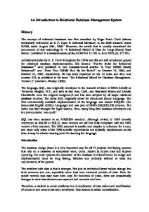
FRANC3D Live Prediction
Crack Propagation
Fracture Analysis
Boundary Conditions
Solid Model
Introduce Flaws
YES NO Acceptable Error?
Unstructured Refinement
Structured Refinement
Volume Mesh
Finite Element Formulation
Increase Order of Basis Functions Estimate Errors
Iterative Solution
Fig. 1. CPTC simulation loop.
• ODBC – “for everything else”. XML figures prominently in ADO.NET, but a discussion is beyond the scope of this brief overview. In all our implementations, described below, we use ADO.NET’s SQL Server .NET data provider defined in the System.Data.SqlClient namespace of the .NET framework.
III. Case Study In this section, we show some preliminary results for a simple computational mechanics application; we solve the equations of linear elasticity for a spiral bevel gear model and a polycrystal. A. The CPTC environment The CPTC environment was developed for NSF’s Crack Propagation on Teraflop Computers (CPTC) project [8] at Cornell University. Figure 1 is a schematic of a lifetime analysis that can be done with CPTC. CPTC supports non-manifold topologies and watertight geometries of polynomial B´ezier curves and patches. The supported finite element shapes are tetrahedra, hexahedra, prisms and pyramids. Originally, the input data (geometry, boundary conditions, mesh) were stored as ASCII or XDR [34] files. The file size, obviously, depends on the topological and geometric complexity of the underlying model, as well as the capabilites of the employed mesh generator. The size of the geometry file, typically, does not exceed a few hundred kilobytes to a few megabytes. The mesh file, on the other hand, can grow almost without limits and is often several hundred megabytes large. There is an augmented version of the mesh format for parallel distributed memory computing, which accounts for partitioning, sharing and ownership of grid entities. A.1 Changes to CPTC First of all, the models are no longer stored in files, but in a RDBMS, Microsoft SQL Server 2000, in this case.
The schema of the underlying database has about 25 tables representing the topological decomposition, geometry (parametrized curves and patches) and tesselation (vertices, tetrahedra etc.). In the previous version of CPTC, a mesh would be partitioned at runtime by invoking METIS [19]. In contrast, the set of tetrahedra is now stored in the database as a partitioned set. The partitioning is fixed by the time the database is created and it is generated from a space-filling curve (Hilbert curve) [28], [14]. Depending on the size of the underlying mesh, the set is split into a maximum number of partitions – 128 in the examples below – and if there are fewer processors available at runtime, the smaller partitions are dynamically combined into larger partitions. For example, MPI process 0 would issue the following SELECT command to retrieve its subset of tetrahedra, if there were only 16 MPI processes total: SELECT * FROM Tetrahedra WHERE partition BETWEEN 0 AND 7 Obviously, we exploit the locality-preserving nature of space-filling curves to ensure that this combination process yields reasonable partitions. The partition column is used to define an appropriate clustered index [9] to speed up the (MPI) client queries, which typically involve only data in the scope of a partition. The read routines for the solution phase now reduce to a few lines of code, basically a few SQL queries (strings). Another set of changes deals with post-processing. The visualization routines (Python and VTK) now talk directly to the database and steering capabilities can be easily implemented as dynamical SQL query generation. Fracture analysis, including stress intensity factor (SIF) calculation and new crack front prediction, was previously performed directly after the solver. Even if a model contains multiple cracks, the parallelism in SIF calculations is negligible and the subset of data required is marginal compared to the size of the entire model. What is expensive (and not problem-oriented) is to extract the relevant data (geometry, mesh and displacements near the crack front) and it seemed natural to do this after the solver, since all data, though scattered across multiple nodes, were present in memory. With a RDBMS as a backend, the fracture analysis can be easily done as a decoupled standalone application that retrieves only the data necessary. Adaptive unstructured re-meshing and quality assessment is much easier to do when the model resides in an RDBMS. B. System Configuration The results shown in subsection III-C were obtained using the following configuration: • A cluster of 64 DELL PowerEdge 1550 servers with two Pentium III@1 GHz, 256 KB L2-cache per processor, 2 GB RAM per node and Giganet interconnect running Windows 2000 Advanced Server (SP2), Microsoft .NET Framework, and MPIPro 1.6.3,
5
MPI processes Read Time (s) Solve Time (s) Write Time (s)
8 5.00 n/a n/a
16 5.30 1,901.73 18.26
32 6.47 955.21 18.26
64 9.30 470.44 18.26
128 14.44 250.37 18.26
MPI processes Read Time (s) Solve Time (s) Write Time (s)
8 22.54 n/a n/a
16 23.25 n/a n/a
32 23.23 n/a n/a
64 23.48 3669.28 143.00
128 25.47 3019.22 143.00
TABLE I Sample results for a for a gear model.
TABLE II Sample results for a polycrystal model.
A single DELL PowerEdge 2450 server with two Pentium III@600 MHz, 256 KB L2-cache per processor, 1 GB RAM, running Windows 2000 Advanced Server (SP2) and a single instance of SQL Server 2000 (SP2). • The cluster is connected to the database server over standard 100 MBit ethernet.
formulation, node numbering and assembly) are provided to put the read/write results in perspective.
•
C. Results Our sample application performs the following steps: 1. Using mpirun we invoke a simple ADO.NET client for each MPI process, which reads this processes sets of tetrahedra, nodes, shared nodes and boundary conditions (Dirichlet and Neumann), and writes them to a node’s local harddisk. 2. mpirun then invokes the program dealing with finite element formulation and assembly, and finally PETSc’s [24], [2] SLES package is called to solve the underlying equations. 3. After the solve is complete the results are written to MPI process 0’s local harddrive and written back by another ADO.NET client to the database. In this application, no interaction with the database occurs during the solve. Since all the results are gathered first by MPI process 0, the time for writing the data to the database does not depend on the number of clients. C.1 Gear Model A model of spiral bevel gear was created using OSM/FRANC3D [7] and discretized using the JMESH [20] mesh generator. The underlying finite element mesh consists of 193,405 T10-elements (10-noded tetrahedra) resulting in a system with 835,851 degrees of freedom. The amount of data to be read from the database is about 7 MB. In Table I, results are shown for a fixed problem size varying the number of clients. The solve times (including formulation, node numbering and assembly) are provided to put the read/write results in perspective. (The RAM of 8 nodes is not sufficient to formulate/solve the underlying system of equations.) C.2 Polycrystal Model A model of 100 grain polycrystal was created using the Digital Material Toolkit [10] and discretized using the QMG [25] mesh generator. The underlying finite element mesh consists of 1,519,816 T10-elements resulting in a system with 6,271,419 degrees of freedom. The amount of data to be read from the database is about 70 MB. In Table II, results are shown for a fixed problem size varying the number of clients. The solve times (including
D. Discussion The dataset underlying Table II is about ten times as big as the one from Table I. Nevertheless, the performance, e.g. the effective bandwidth, for different numbers of clients is better for the larger database. The overhead for connection management exceeds the data transfer time for small datasets. The updates are fairly slow. A linked server (see Section IV) can improve this somewhat, but it remains a problem. Overall we spend about 10% of the total execution time for I/O, which is an acceptable number and comparable to file based approaches, when factoring in the partitioning time etc. There is plenty of room for improvements: some of the data in the database can be easily recalculated and this is preferable if it significantly cuts down on the amount of data that is read/written at runtime. The use of clustered indexes clearly pays off. With too many clients a single database server becomes a bottleneck and a single point of failure. The scenario outlined above is clearly inadequate for hundreds of MPI clients. In the next section we describe how to deal with the problem of scaling out. This simple example highlights only the part that is critical for the solution process. Typically, finite element applications have extensive pre- and postprocessing phases (error analysis, visualization) which operate on small (changing) subsets of data. This is a major source of non-problemoriented code in applications, and this is where the power of SELECT and the superior interoperability of an RDBMS come to bear. The migration from a file based environment to a RDMBS was relatively straightforward. Besides code reduction we had to add some code as “glue” for those applications that do not (yet) talk directly to the database, but via a Python or C# wrapper. The overall design is one of greater modularity and robustness. Having our models in a database, makes it a lot easier to read and write data in third party formats. For instance, it is fairly straightforward to create a script that writes parts of or an entire model in a given format. This approach is certainly preferable to maintaining a zoo of conversion routines. Caution: We do not claim that using databases is appropriate in every sitution. They are probably not appropriate when the ultimate level of performance is the goal and very high development costs are budgeted. Also, if the
6
underlying data are regular and structured and no datamining type functionality is needed, not much benefit can be expected from an RDBMS beyond the transactional capabilities and interoperability. IV. Future Work We will leverage the fact that our application uses databases in order to investigate the following: • Scalability, • Fault-tolerance, • Distributed computing and Web services. All current generation commercial RDBMS from vendors like IBM, Microsoft or Oracle support SMP architectures with some form of multiprocessing or multithreading. One can either run multiple instances of the RDBMS in one SMP and/or rely on the server engine’s ability to extract parallelism from the queries and dynamically spawn processes or threads. Scalability can be enhanced and throughput increased by adding faster processors, more memory, faster disks and so on. This scale-up approach is restricted by the inherent limitations of the SMP model, the ability of the server engine to extract parallelism, as well as the bandwith and latency limits of the network interface(s). If we plan on serving hundreds of MPI processes off a (logically) single large database, it is rather unlikely that SMPtype scalability will be sufficient. (If the database to be served is relatively small, we could just replicate it across multiple servers and this solution would be, except for updates, almost infinitely scalable.) With distributed partitioned views [9] Microsoft’s SQL Server 2000 supports the notion of data partitioned over multiple servers. Roughly speaking, a distributed partitioned view makes data residing in tables across multiple servers appear as if they come from a single table. With this scale-out approach, almost linear scalability can be achieved, assuming that the data easily lend themselves to partitioning. For an excellent discussion of the technical details we refer the reader to [3]. Related results will be reported elsewhere. We have begun to deploy many of our applications as Web services [29]. Mesh generation and solver components, for example, are good candidates for such services. However, the potentially large input data and/or return objects do not fit the simple “given the zip code, return temperature” picture. There are problems related to scheduling, data staging, discovery, transfer and transformation that need to be addressed. Given their interoperability characteristics we think that traditional RDBMS and “virtual databases” like Astrolabe [26] are poised to fill in this gap. Using this paradigm, as a proof-of-concept we plan to deploy a distributed simulation involving chemically reacting flows, heat transfer and fracture mechanics in late summer this year. V. Conclusions In addition to being competitive with file based approaches, RDBMS offer a key advantage: they yield a dramatic reduction of non-problem-oriented code. With SQL as a data definition language it is easy to ensure consistency
of data and their referential integrity. On the other hand, since SQL is a powerful data manipulation language, it is cheap to prototype and change data-access API’s (SQL commands are just human readable strings.) A greater level of fault tolerance, high availability and interoperability comes on top of that (without additional coding). Depending on the nature and size of the underlying data, different approaches like replication or partitioning can be taken to achieve scalability. Files remain indispensible as temporary storage, but are completely inadequate as persistent and intelligent storage for building distributed applications around large datasets. Acknowledgments The authors would like to thank Jim Gray of Microsoft Research for his support and many helpful suggestions. We gratefully acknowledge the support of Microsoft Research, Dell, Microsoft and Intel. References [1] ITR/ASP: Adaptive Software Project Home Page, http://www.erc.msstate.edu/ jcollins/ITR/index.html [2] Satish Balay et al., PETSc Users Manual, ANL-95/11 - Revision 2.1.1, Argonne National Laboratory, 2001. [3] Itzik Ben-Gan and Tom Moreau, Advanced Transact-SQL for SQL Server 2000, Apress, 2000. [4] Joe Celko, SQL for Smarties: Advanced SQL Programming, Morgan Kaufmann Publishers, 2000. [5] Paul Chew, Proposal for Database Schema for ASP Geometries, Cornell University, January 2002. [6] Paul Chew, Proposal for Database Schema for ASP Generalized Meshes, Cornell University, January 2002. [7] Cornell Fracture Group Home Page, http://www.cfg.cornell.edu/software/CFG software.html [8] Crack Propagation on Teraflop Computers, http://www.tc.cornell.edu/Research/CMI/CrackProp/index.asp [9] Kalen Delaney, Inside Microsoft SQL Server 2000, Microsoft Press, 2001. [10] Digital Material Toolkit, http://www.tc.cornell.edu/Research/ CompMatSci/Multiscale/DigitalMaterial/ [11] Jack J. Dongarra and David W. Walker, The Quest for Petascale Computing, Computing in Science and Engineering, May/June 2001, IEEE 2001. [12] Flow Analysis Software Toolkit (FAST), http://www.nas.nasa.gov/Software/FAST/ [13] Ben Forta, Sams Teach Yourself SQL in 10 Minutes, Sams, 2001. [14] Michael Griebel and Gerhard Zumbusch, Hash-Storage Techniques for Adaptive Multilevel Solvers and Their Domain Decomposition Parallelization, Contemporary Mathematics, Vol. 218, 1998. [15] John Griffin, XML and SQL Server 2000, New Riders Publishing, 2001. [16] Gerd Heber, David Lifka and Paul Stodghill, Post-Cluster Computing and the Next Generation of Scientific Applications, To appear, 2002. [17] JDBC Technology, http://java.sun.com/products/jdbc/ [18] Wei-Meng Lee, The Evolution of Data-Access Technologies, SQL Server Magazine, Vol. 4, No. 4, pp. 28–34, April 2002. [19] METIS: Family of Multilevel Partitioning Algorithms, http://www-users.cs.umn.edu/ karypis/metis/ [20] J. B. Cavalcante Neto et al., An Algorithm for ThreeDimensional Mesh Generation for Arbitrary Regions with Cracks, Engineering with Computers (2001) 17, 75–91. [21] ODBC 3.0 Software Development Kit and Programmer’s Reference, Microsoft Press, 1997. [22] Microsoft OLE DB, http://www.microsoft.com/data/oledb/ default.htm [23] Michael Otey and Paul Conte, SQL Server 2000 Developer’s Guide, Osborne/McGraw-Hill., 2001. [24] PETSc home page, http://www.mcs.anl.gov/petsc/
7
[25] QMG 2.0 home page, http://www.cs.cornell.edu/Info/People/ vavasis/qmg2.0/qmg2 0 home.html [26] Robbert van Renesse and Kenneth Birman, Astrolabe: A Robust and Scalable Technology for Distributed System Monitoring, Management and Data Mining, http://www.cs.cornell.edu/Info/Projects/Spinglass/public pdfs/ Astrolabe.pdf [27] David F. Rogers, An Introduction to NURBS With Historical Perspective, Morgan Kaufmann Publishers, 2001. [28] Hans Sagan, Space-Filling Curves, Springer-Verlag, 1994. [29] Web Services, http://www.w3.org/2002/ws/ [30] W. Z. Strang, Cobalt60 : User’s Manual, Air Force Research Laboratory, Wright-Patterson AFB, OH, September 2000. [31] Andrew Trice, Connect to Microsoft SQL 2000 with the Perl Sybase Module, LINUX Journal, April 2002, pp. 62–65. [32] Steve Vavasis, Proposal for Geometric Representation, Cornell University, October 2001. [33] Steve Vavasis, Proposal for Boundary Condition and Material Property Representation, Cornell University, October 2001. [34] XDR: External Data Representation Standard, http://www.faqs.org/rfcs/rfc1014.html [35] Extensible Markup Language (XML), http://www.w3.org/XML/