Loopy BP came out of the study of Bayesian networks2 [13, 3, 5]. Pearl proposed ... singly connected, i.e. no loop appears when viewed as an undirected graph,.
Linkoping Electronic Articles in
Computer and Information Science Vol. n(2002): nr nn
Computing Kikuchi approximations by Cluster BP Taisuke Sato Department of Computer and Information Science Tokyo Institute of Technology / CREST Tokyo, Japan
Linkoping University Electronic Press Linkoping, Sweden
http:/ /www.ep.liu.se/ea/cis/2002/nnn/
Published on February nn,, 2002 by Linkoping University Electronic Press 581 83 Linkoping, Sweden Link oping Electronic Articles in Computer and Information Science
ISSN 1401-9841 Series editor: Erik Sandewall
c 2002 Taisuke Sato Typeset by the author using LATEX Formatted using �etendu style Recommended citation:
. . Linkoping Electronic Articles in
Computer and Information Science, Vol. n(2002): nr nn.
http://www.ep.liu.se/ea/cis/2002/nnn/. February nn,, 2002.
This URL will also contain a link to the author's home page. The publishers will keep this article on-line on the Internet (or its possible replacement network in the future) for a period of 25 years from the date of publication, barring exceptional circumstances as described separately. The on-line availability of the article implies a permanent permission for anyone to read the article on-line, to print out single copies of it, and to use it unchanged for any non-commercial research and educational purpose, including making copies for classroom use. This permission can not be revoked by subsequent transfers of copyright. All other uses of the article are conditional on the consent of the copyright owner. The publication of the article on the date stated above included also the production of a limited number of copies on paper, which were archived in Swedish university libraries like all other written works published in Sweden. The publisher has taken technical and administrative measures to assure that the on-line version of the article will be permanently accessible using the URL stated above, unchanged, and permanently equal to the archived printed copies at least until the expiration of the publication period. For additional information about the Linkoping University Electronic Press and its procedures for publication and for assurance of document integrity, please refer to its WWW home page: http://www.ep.liu.se/ or by conventional mail to the address stated above.
Abstract In this paper, we investigate loopy BP (belief propagation) which is at the crossroads of Bayesian networks, statistical physics and error correction decoding. It is a method of computing exact and approximate marginals based on a minimization of variational free energy, and o�ers a quite powerful means for otherwise computationally intractable problems. We re-examine its theoretical background, the Kikuchi approximation, and propose Cluster BP, a mild generalization of loopy BP that can compute some class of Kikuchi approximations. We also propose Cluster CCCP as a convergent version of Cluster BP to compute local minima of Kikuchi approximations.
1
1
Introduction
In this paper, we investigate1 loopy BP (belief propagation) which is at the crossroads of Bayesian networks, statistical physics and error correction decoding. It is a method of computing exact and approximate marginals based on the minimization of variational free energy, and o�ers a quite powerful means for otherwise computationally intractable problems. Loopy BP came out of the study of Bayesian networks2 [13, 3, 5]. Pearl proposed the BP (belief propagation) algorithm for computing marginal distributions [12]. It is a message passing algorithm that propagates messages (probability distributions) over a Bayesian network. When the network is singly connected, i.e. no loop appears when viewed as an undirected graph, it computes exact marginals in time linear in the size of the network [12].3 As BP is just a local message passing algorithm, it is applicable even when the network contains loops (hence the name \loopy BP"), though at the risk of non-convergence. Historically while what loopy BP does was obscure in the case of loopy networks, experiments revealed that it is very versatile and e�ective, and sometimes can give remarkably good approximate marginals especially when used for error correction decoding [8, 10, 18]. It was not until recently that Yedidia et al. discovered that what loopy BP actually does is computing a stationary point of a certain quantity known as the Bethe approximation to the free energy in statistical physics [19]. The Bethe approximation is just one of the possible approximations to the free energy. Yedidia et al. proposed GBP (generalized BP), a new message passing algorithm that yields, when it converges, a stationary point of the Kikuchi approximation which is more complicated but more accurate than the Bethe approximation as a generalization of the Bethe approximation [9, 19].4 Yuille proposed an alternative to GBP, CCCP double-loop algorithm5 , that is guaranteed to converge to local minima of the Bethe and Kikuchi approximations. This convergence property is achieved by his new optimizing technique for the class of functions decomposable as a sum of convex and concave functions [21]. While loopy BP is only able to compute stationary points of Bethe approximations, it is simple and e�cient. Contrastingly GBP and CCCP for Kikuchi approximations are quite general but rather complex. In this 1 Our investigation is motivated by PRISM, a general symbolic-statistical modeling language which we have been developing for years [14, 16, 17]. It is based on a rigorous mathematical semantics and enables one to build a complex statistical model as a PRISM program and e�ciently learn parameters embedded in the program through the graphical EM algorithm [15, 17]. The computational e�ciency is achieved however by restricting programming style so that it complies with assumptions of probability computation employed by PRISM. We are seeking for a general yet robust method of probability computation to realize more freedom of PRISM programming. 2 A Bayesian network is a nite directed acyclic graph representing probabilistic causal relationships between random variables. Vertices are random variables which are connected by directed edges from parent vertices to child vertices. A conditional distribution p(X = x j Y1 = y1 ; : : : ; Ym = ym ) (m � 0) is associated with each vertex X and its parents Y1 ; : : : ; Ym . The graph de nes a joint distribution as a product of these conditional distributions. 3 For Bayesian networks which are not singly connected, the junction tree algorithm [7] is available to e�ciently compute marginal distributions. 4 Descriptions of the Bethe and Kikuchi approximations in this paper are largely due to [19]. 5 \CCCP" stands for the Concave-Convex Procedure.
2 paper, we take an intermediate approach. Keeping the simplicity of loopy BP, we extend it to the Cluster BP algorithm allowing messages to contain more than one variable so that it can compute Kikuchi approximations when a certain condition is satis ed. Furthermore, to remove the possibility of non-convergence, we derive the Cluster CCCP algorithm following Yuille's convex-concave decomposition. It always converges and gives the same result as the Cluster BP algorithm. In the sequel, we rst quickly review the problem to be solved. We then introduce the Kikuchi approximation in a slightly generalized form by dropping the requirement that clusters used in the approximation must be closed under intersection. We also introduce a class of undirected labeled graphs called cluster graphs. After these preparations, two new algorithms, Cluster BP and Cluster CCCP, are proposed which run on cluster graphs. Both compute stationary points of (generalized) Kikuchi approximations but the latter is convergent and guaranteed to compute a local minimum. The reader is assumed to be familiar with Bayesian networks and the junction tree algorithm [4, 3].
2
Preliminaries
2.1
Variable free energy
We assume a discrete random vector X = (X1 ; : : : ; Xn ) of n dimension is given and has a joint distribution p(x) = p(x1 ; : : : ; xn ) such that
� p(x) is always positive, p(x) > 0 for any x. � p(x) is presented as a product of positive functions potential s.
p(x) = � = where E (x) def =
Y
� (x� ) �2P 1 0E(x) e
(1)
Z
X
�2P
0 ln
� (x� )
Z def = �01 =
� (x� ) called
XY
x �2P
(2) (3)
� (x � )
Here � is a normalizing constant and Z is a partition function. E (x) is considered to be the \energy" of a state x. We call each i (1 � i � n) a variable index. Let � denote a sub-vector of (1; : : : ; n), the vector of all variable indecies, and P be a collection of such sub-vectors. x� then stands for a sub-vector of (x1 ; : : : ; xn ) corresponding to �. For instance, if x = (x1; x2; x3 ; x4 ) and � = (2; 4), we have x� = (x2; x4). For convenience, we identify a sub-vector � = (i1 ; : : : ; ik ) (1 � k � n) with the set fi1 ; : : : ; ik g like � = (2; 4) = f2; 4g. Because both notations are mutually convertible, such treatment does not cause confusion. A non-empty subset � of f1; : : : ; ng is called a cluster and if � is in P, it is referred to as a potential cluster. When � and are clusters, so are � \ ,
3
� [ and � n . Operations on clusters re ect on vectors. For example, put � = f1; 2; 3g and = f2; 3; 4g. Then x�\ = xf2;3g = (x2 ; x3 ) and x�n = xf1g = x1. A � B means A is a proper subset of B whereas A � B means A � B or A = B . We de ne the variational free energy F (b) w.r.t. the energy E (x) by F (b) def = (average energy) 0 (entropy) X X = b(x)E (x) + b(x) ln b(x) x
x
where b(1) is a test distribution. Because F (b) = P
�
P
(4) �
b(x) x�b(x) ln p(x)
�
0 ln Z
and the Kullback-Leibler divergence x b(x) ln pb((xx)) is non-negative and zero only when b(1) = p(1), F (b) takes a minimum value if and only if b(1) = p(1). In other words, we have an equation p = argminb F (b). Suppose a distribution p(x) is given by (1). For the variational free energy F (b), we can de ne its approximation, the Kikuchi approximation FK (fb�g) such that F (b) � FK (fb� g).6 Combining the Kikuchi approximation with p = argminb F (b), we obtain an approximation scheme for marginal distributions fp�(x� )g of p(x):
fp� g �
argminfb� g FK (fb� g):
We read this equation from right to left and calculate approximate marginal distributions fp� g by minimizing the functional FK (fb� g) with respect to fb�g as variational variables. In view of the signi cance of computing marginals in many elds including pattern recognition, natural language processing, robotics, bioinformatics, coding theory etc on one hand and the di�culty of their exact computation on the other hand, it is quite important to develop e�cient algorithms for computing argminfb� g FK (fb� g). The objective of this paper is to propose such algorithms while preserving the simplicity of BP. 2.2
The Kikuchi approximation
In this subsection, we introduce the Kikuchi approximation [9, 19] in a slightly generalized form. Let P be a set of potential clusters appearing in (1). For P we introduce another set U of clusters such that
�
for any � in P, there exists the smallest 2 U that includes �, i.e. � � and if 0 � � then 0 � for any 0 2 U.7
is called a set of clusters for P. We consider U as a partially ordered set ordered by set inclusion ordering. Let B be the set of maximal clusters in U. If U is generated from B by taking all possible non-empty intersections of elements in B, i.e. U = f�1 \ : : : \ �h j �i 2 B; 0 < h; 1 � i � hg, a cluster in U is called a Kikuchi cluster, and U a set of Kikuchi clusters for P. We associate an overcounting number a� with a cluster � in U which is inductively de ned from maximal clusters as follows[9, 19]. U
6 b� (x� ) (resp. p� (x� ) ) denotes a marginal distribution of b(x) (resp. p(x)) marginalized to x� . 7 This condition is trivially satis ed by putting U = P, but for the sake of freedom of approximations, we prefer to introduce U independently of P.
4
(
a� def = 1 if � is maximal in U P def a� = 1 0 : ��; 2U a o.w.
By de nition
X
�:�2U;�� P
a� = 1 for 8 2 U:
Introduce E�+ (x� ) def = 0 ln � (x�) and transform the average energy b ( x ) E ( x ) using the above property of overcounting numbers as follows. x X
x
b(x)E (x) = = = =
Here b (x ) def =
P
X
b(x)
x
X
: 2P
X X
: 2P x
b (x )E + (x )
0
X
E +(x )
X
@
: 2P �2U;�� X
�2U
a�
X
x�
x[n]n b(x) ([n] = P
1
a� A
X
x
b (x )E +(x )
b�(x� )E�(x� )
f1; : : : ; ng)
(5)
is a marginal distribu-
tion and E� (x�) = : 2P; �� E + (x ) is the energy of cluster �. Now the average energy is expressed as a linear combination of average cluster energies. P It is unfortunate that a similar transformation of the entropy S = 0 x b(x) ln b(x) is impossible because of non-linearity of the entropy function. Yet we can derive its approximation as a linear combination of cluster entropies. First introduce S�, the entropy of a cluster � by def
S� def =0
X
x�
b� (x�) ln b�(x� ):
Inductively de ne S�+ from minimal elements of U by (
S�+ def = S� if � is minimal in U P def + S� = S� 0 : ��; 2U S + o.w.
For every � 2 U, we have
X
S� = Accordingly if we assume S �
S
� =
P
: ��; 2U
S +:
+ 8 2U S , we see
X
2U X
2U X
S + 0 @
X
�2U;��
1
a�A S +
a� S � : (6) �2U 8 This assumption is justi ed empirically in statistical physics. The reader is advised to see [9] for the development of the Kikuchi approximation. =
5 Putting (5) and (6) together, the variational free energy F (b) is approximated as follows.
F (b) =
�
X
x
b(x)E (x) +
X
�2U
X
a�
x�
X
x
b(x) ln b(x)
b� (x� )E�(x� ) +
X
x�
!
b�(x� ) ln b� (x�)
We de ne the generalized 9 Kikuchi approximation F~K (fb�g) for F (b) by
F~K (fb� g) =
def
= where �� (x�)
X
�2U X
�2U
X
a� a�
x�
X
x�
b�(x� )E�(x� ) +
b� (x� ) ln
= e0E� (x� )
�
b � (x � ) �� (x� )
X
x�
�
!
b�(x� ) ln b� (x�) (7)
def
0
= exp @
1
X
: 2P; ��
=
Y
: 2P; ��
0E +(x )A
(x ):
(8)
When U is a set of Kikuchi clusters for P, F~K (fb�g) is identical to the Kikuchi approximation de ned in [19]. The Bethe approximation is a special case of the Kikuchi approximation where U is a union of clusters B of the form fi; j g (i 6= j ) and a set of intersections f�1 \ �2 j �1 ; �2 2 Bg.
3
Cluster graphs
Just like Pearl's BP runs on Bayesian networks and the junction tree algorithm runs on junction trees, our new algorithms, Cluster BP and Cluster CCCP, run on cluster graph s which can be seen as a generalization of junction trees to graphs and also can be seen as a re nement of \junction graphs" [2] with a partial ordering over clusters and a suitable condition for computing the Kikuchi approximation. From here on for brevity, we interchangeably use n1 1 1 1 nh for cluster fn1 ; : : : ; nh g like 123 for f1; 2; 3g. Let U be a set of clusters for P. A labeled undirected graph GU is said to be a cluster graph for U if vertices and edges are labeled by clusters in 10 U as follows and if there is such a graph, we say U has a cluster graph.
�
Every maximal element in of a vertex.
U
appears exactly once in GU as a label
9 The term \generalized" is added to make clear the distinction between the Kikuchi approximation de ned in [19] and the one de ned here which does not require U to be closed under intersection. 10 U may not have a cluster graph. For instance U1 = f1467; 2457; 3567; 47; 57; 67g has a cluster graph but U2 = U1 [ f7g has no cluster graph. If the Hasse diagram HU of U is a tree, then HU is a cluster graph for U. In general however, nding an e�cient algorithm for the construction of cluster graphs is a future research topic.
6
� �
Suppose vertices v1 and v2 are respectively labeled �1 and �2 . The edge connecting v1 and v2 , if any, is labeled � �1 \ �2 ( 6= ;). When the equality = �1 \ �2 holds for every label on an edge, we say GU is regular. The tree condition is satis ed: for every � 2 U, the subgraph of GU consisting only of the vertices and edges whose label include � is a tree.
Please note that we allow the same cluster to occur (as a label) more than once in a cluster graph. So vertices and edges can be labeled by a common cluster. By the way it is obvious that junction trees are cluster graphs such that nodes are cliques and the tree condition is satis ed. We have a look at examples of cluster graphs. 12 34
16 8
23
14
23 12 34 5
12 4
18 14 78
5
14
24
8 23 12 34 4
58 9
13 4
34
(B) The tree condition violated w.r.t. U B
(A) The tree condition satisfied w.r.t. U A
Figure 1: The left graph (A) satis es the tree condition w.r.t. The right graph (B) violates the tree condition w.r.t. UB .
U
A
.
The left graph (A) in Figure 1 is a cluster graph for UA = f1234; 2356; 589; 1478; 168; 14; 18; 23; 1; 5; 8g. It is regular. The maximal clusters are BA = f1234; 2356; 589; 1478; 168g. Since their intersections yield UA , UA is a set of Kikuchi clusters for P = BA . Associated overcounting numbers are a1234 = 1 1 1 = a168 = 1 for the maximal clusters, a23 = a5 = a8 = a14 = a18 = 01 and a1 = 0 for the rest. We check the tree condition. For example the subgraph comprised of vertices and edges that include cluster 23 is a tree. Similarly, the one containing 1, though it does not appear as a label, is also a tree and so on. So (A) satis es the tree condition. The right graph (B) however does not satis es the tree condition w.r.t. UB = f124; 234; 134; 14; 24; 34; 4g because all vertices and edges include 4 and they form a loop. (B) is not a cluster graph for UB (instead it is a cluster graph for U0B = UB n f4g). 24 14 4
24
34
4 4
14
34
(C)
4
4
4
4 4
(D)
Figure 2: Cluster graphs with a multiple occurrence of the same label In Figure 2 both (C) and (D) are cluster graphs for the same cluster set UC = f14; 24; 34; 4g.
7 We next prove a proposition that states the relationship between the tree condition and overcounting numbers. Proposition 3.1
Let GU be a cluster graph for U and a� an overcounting number of � 2 U. Also let V (�) and E (�) respectively be
V (�) def = the number of vertices whose label is � def E (�) = the number of edges whose label is �. We have a� = V (�) 0 E (�).
(Proof) By induction the size of clusters. Suppose � is a maximal cluster. Then there is exactly one vertex labeled � whereas there is no edge labeled � by the tree condition. So V (�) 0 E (�) = 1 = a� . Now suppose the proposition holds for all � �.
a� = 1 0 = 10 (
X
:�� 2U X
:�� 2U
a (V ( ) 0 E ( )) )
(
)
the number of edges the number of vertices = whose label properly 0 whose label properly + 1 include � include � Recalling that the following holds by the tree condition ( ) the number of vertices V (�) + whose label properly include ( � ) the number of edges = E (�) + whose label properly + 1 include � = V (�) 0 E (�) Q.E.D. Proposition 3.2
Suppose U has a cluster graph. Then for every � 2 U, a� � 0 if � is not maximal in
U
.
(Proof) Let � be a non-maximal element in U. There is a maximal 2 such that � � . If no vertex bears � as a label, then a� � 0 by Proposition 3.1. Suppose otherwise and a vertex v is labeled by �. Due to the tree condition, there is a path connecting v and w where w is the vertex labeled by . Let u, 0 and respectively be a vertex on the path adjacent to v , its label and the label of the edge connecting u and v. We have � � 0 and � � because all vertices and edges on the path have a label containing �. On the other hand, due to the labeling condition, � � \ 0 = �. Hence
= �. We may assume 0 6= � (o.w. we merge u and v and their labels 0 ). So there is a map from the vertex v labeled � and its edge labeled � connecting to an adjacent node whose label is not �. Consequently, from Proposition 3.1, we conclude a� � 0. Q.E.D. U
We remark that \overcounting numbers of non-maximal clusters are not positive" is a necessary condition for the tree condition but not a su�cient condition.
8
4
Cluster BP
In this section, we derive an iterative algorithm, Cluster BP, running on cluster graphs which computes a stationary point of the generalized Kikuchi approximation by exchanging messages between vertices in a cluster graph. 4.1
Deriving Cluster BP
We restate our assumptions and notational conventions.
�
�
Q
A joint distribution p(x) = � �2P � (x� ) is speci ed by using potential clusters P and potentials � (x� ). Potentials are always positive. We aim is to e�ciently compute approximate marginals fp�(x� )g by minimizing the generalized Kikuchi approximation F~K (fb� g) de ned by (7). is a set of clusters for P. �� (x�) is the �'s potential de ned by Q ��(x� ) def = : 2P; �� (x ).
U
� GU
is a cluster graph for U. We denote by V (resp. E ) the set of vertices (resp. edges) in GU , and by v (resp. by e) the cluster labeling a vertex v 2 V (resp. the cluster labeling an edge e 2 E ).
Now back to the generalized Kikuchi approximation F~K (fb� g). We rewrite it using Proposition 3.1 as follows.
F~K (fb� g) =
�
b (x ) a� b� (x� ) ln � � � � (x � ) x� �2U X
X
� �
�
b (x ) = (V (�) 0 E (�)) b� (x� ) ln � � � � (x� ) x� �2U � � X X b (x ) = V (�) b�(x� ) ln � � � � (x� ) x� �2U � � X X b� (x�) 0 E (�) b�(x� ) ln � (x ) � � x� �2U � � XX � � XX bv (xv ) b e (x e ) = bv (xv ) ln 0 be (xe ) ln �v (xv ) �e(xe ) v2V xv e2E xe X
X
Note the last equation is expressed solely in terms of marginal distributions fbv (xv ); be(xe )g that correspond to labels of vertices and edges in GU . We minimize F~K (fb�g) as a functional over fbv (xv ); be (xe )g to obtain approximate marginals but the minimization must be carried out under two constraints. Distribution: Consistency:
P
P
xv bv (xv ) = 1 for every vertex v .
xvne bv (xv ) = be(xe ) for every vertex
v and its edge e.11
For any clusters ; � ( � �), the tree condition guarantees the existence of a path connecting and � regardless of whether they label a vertex or not. P Hence, if the consistency holds along this path, x�n b� (x� ) = b (x ) must hold transitively. 11
9 So we introduce a Lagrangian L = FK (fbv (xv ); be (xe )g)+C with a constraint term C .
C
def
=
8 0 1 X XX< e �v (xe ) @ bv1 (xv1 ) be (xe )A : 1 xv1 ne e 2E x e 0 0 19 = X X X e +�v2 (xe ) @ bv2 (xv2 ) be (xe )A + �v @ bv (xv ) ; xv xv2 ne v2V
0
0
1
0 1A
One thing must be noted here. Setting the derivatives of L with respect to fbv (xv ); be(xe )g equal to zero does not give an algorithm which exchanges messages among vertices because L's variational variables correspond to la-
bels of vertices, not to vertices themselves (some vertices may have a common label). We therefore in ate variational variables by introducing new variables fbv (xv ); be (xe )g which have one-to-one correspondence to vertices v and edges e.12 However this change does not a�ect the solution because the tree condition ensures that those vertices or edges with a common label will have the same distribution. So our nal Lagrangian becomes
L0
= F~K0 + C 0
F~K0 =
XX
v2V xv
bv (xv ) ln
�
b v (x v ) � v (x v )
b (x ) = bv (xv ) ln v0 v � v (x v ) v2V xv XX
C0
=
8 XX