Cluster Identi’ cation Using Projections Daniel Peña and Francisco J. Prieto This article describes a procedure to identify clusters in multivariate data using information obtained from the univariate projections of the sample data onto certain directions. The directions are chosen as those that minimize and maximize the kurtosis coef cient of the projected data. It is shown that, under certain conditions, these directions provide the largest separation for the different clusters. The projected univariate data are used to group the observations according to the values of the gaps or spacings between consecutive ordered observations . These groupings are then combined over all projection directions. The behavior of the method is tested on several examples, and compared to k-means, MCLUST, and the procedure proposed by Jones and Sibson in 1987. The proposed algorithm is iterative, af ne equivariant, exible, robust to outliers, fast to implement, and seems to work well in practice. KEY WORDS: Classi cation; Kurtosis; Multivariate analysis; Robustness; Spacings.
1.
INTRODUCTION
Let us suppose we have a sample of multivariate observations generated from several different populations. One of the most important problems of cluster analysis is the partitioning of the points of this sample into nonoverlapping clusters. The most commonly used algorithms assume that the number of clusters, G, is known and the partition of the data is carried out by maximizing some optimality criterion. These algorithms start with an initial classi cation of the points into clusters and then reassign each point in turn to increase the criterion. The process is repeated until a local optimum of the criterion is reached. The most often used criteria can be derived from the application of likelihood ratio tests to mixtures of multivariate normal populations with different means. It is well known that (i) when all the covariance matrices are assumed to be equal to the identity matrix, the criterion obtained corresponds to minimizing tr4W5, where W is the within-groups covariance matrix, this is the criterion used in the standard k-means procedure; (ii) when the covariance matrices are assumed to be equal, without other restrictions, the criterion obtained is minimizing —W— (Friedman and Rubin 1967); (iii) when the covariance matrices are allowed to be different, the criterion P obtained is minimizing G jD1 nj log Wj =nj , where Wj is the sample cross-product matrix for the jth cluster (see Seber 1984, and Gordon 1994, for other criteria). These algorithms may present two main limitations: (i) we have to choose the criterion a priori, without knowing the covariance structure of the data and different criteria can lead to very different answers; and (ii) they usually require large amounts of computer time, which makes them dif cult to apply to large data sets. Ban eld and Raftery (1993), and Dasgupta and Raftery (1998) have proposed a model-based approach to clustering that has several advantages over previous procedures. They assume a mixture model and use the EM algorithm to estimate the parameters. The initial estimation is made by hierarchical agglomeration. They make use of the spectral decomposition of the covariance matrices of the G populations to allow some groups to share characteristics in their covariance matrices Daniel Peña (E-mail:
[email protected]) is Professor and Francisco J. Prieto (E-mail:
[email protected]) is Associate Professor in Dept. Estadística y Econometrica, Univ. Carlos III de Madrid, Spain. We thank the referees and the Associate Editor for their excellent comments and suggestions, that have improved the contents of this article. This research was supported by Spanish grant BEC2000-0167 .
(orientation, size, and shape). The number of groups is chosen by the B IC criterion. However, the procedure has several limitations. First, the initial values have all the limitations of agglomerative hierarchical clustering methods (see Bensmail and Celeux 1997). Second, the shape matrix has to be speci ed by the user. Third, the method for choosing the number of groups relies on regularity conditions that do not hold for nite mixture models. More exibility is possible by approaching the problem from the Bayesian point of view using normal mixtures (Binder 1978) and estimating the parameters by Markov Chain Monte Carlo methods (see Lavine and West 1992). These procedures are very promising, but they are subject to the label switching problem (see Stephens 2000 and Celeux, Hurn, and Robert 2000 for recent analysis of this problem) and more research is needed to avoid the convergence problems owing to masking (see Justel and Peña 1996) and to develop better algorithms to reduce the computational time. The normality assumption can be avoided by using nonparametric methods to estimate the joint density of the observations and identifying the high density regions to split this joint distribution. Although this idea is natural and attractive, nonparametric density estimation suffers from the curse of dimensionality and the available procedures depend on a number of parameters that have to be chosen a priori without clear guidance. Other authors (see Hardy 1996) have proposed a hypervolume criterion obtained by assuming that the points are a realization of a homogeneous Poisson process in a set that is the union of G disjoint and convex sets. The procedure is implemented in a dynamic programming setting and is again computationally very demanding. An alternative approach to cluster analysis is projection pursuit (Friedman and Tukey 1974). In this approach, lowdimensional projections of the multivariate data are used to provide the most interesting views of the full-dimensional data. Huber (1985) emphasized that interesting projections are those that produce nonnormal distributions (or minimum entropy) and, therefore, any test statistic for testing nonnormality could be used as a projection index. In particular, he suggested that the standardized absolute cumulants can be useful for cluster detection. This approach was followed by Jones and Sibson (1987) who proposed to search for clusters by
1433
© 2001 American Statistical Association Journal of the American Statistical Association December 2001, Vol. 96, No. 456, Theory and Methods
1434
Journal of the American Statistical Association, December 2001
maximizing the projection index I4d5 D Š23 4 d5 C Š24 4 d5=41 where Šj 4 d5 is the jth cumulant of the projected data in the direction d. These authors assumed that the data had rst been centered, scaled, and sphered so that Š1 4 d5 D 0 and Š2 4d5 D 1. Friedman (1987) indicated that the use of standardized cumulants is not useful for nding clusters because they heavily emphasize departure from normality in the tails of the distribution. As the use of univariate projections based on this projection index has not been completely successful, Jones and Sibson (1987) proposed two-dimensional projections, see also Posse (1995). Nason (1995) has investigated three-dimensional projections, see also Cook, Buja, Cabrera, and Hurley (1995). In this article, we propose a one-dimensional projection pursuit algorithm based on directions obtained by both maximizing and minimizing the kurtosis coef cient of the projected data. We show that minimizing the kurtosis coef cient implies maximizing the bimodality of the projections, whereas maximizing the kurtosis coef cient implies detecting groups of outliers in the projections. Searching for bimodality will lead to breaking the sample into two large clusters that will be further analyzed. Searching for groups of outliers with respect to a central distribution will lead to the identi cation of clusters that are clearly separated from the rest along some speci c projections. In this article it is shown that through this way we obtain a clustering algorithm that avoids the curse of dimensionality, is iterative, af ne equivariant, exible, fast to implement, and seems to work well in practice. The rest of this article is organized as follows. In Section 2, we present the theoretical foundations of the method, discuss criteria to nd clusters by looking at projections, and prove that if we have a mixture of elliptical distributions the extremes of the kurtosis coef cient provide directions that belong to the set of admissible linear rules. In the particular case of a mixture of two multivariate normal distributions, the direction obtained include the Fisher linear discriminant function. In Section 3, a cluster algorithm based on these ideas is presented. Section 4 presents some examples and computational results, and a Monte Carlo experiment to compare the proposed algorithm with k-means, the Mclust algorithm of Fraley and Raftery (1999) and the procedure proposed by Jones and Sibson (1987). 2.
CRITERIA FOR PROJECTIONS
We are interested in nding a cluster procedure that can be applied for exploratory analysis in large data sets. This implies that the criteria must be easy to compute, even if the dimension of the multivariate data, p, and the sample size, n, are large. Suppose that we initially have a set of data S D 4X1 1 : : : 1 Xn 5. We want to apply an iterative procedure where the data are projected onto some directions and a unidimensional search for clusters is carried out along these directions. That is, we rst choose a direction, project the sample onto this direction, and we analyze if the projected points can be split into clusters along this rst direction. Assuming that the set S is split into k nonoverlapping sets S D S1 [ S2 [ ¢ ¢ ¢ [ Sk ,
where Si \ Sj D ™ 8 i1 j, the sample data is projected over a second direction and we check if each cluster Si 1 i D 11 : : : 1 k, can be further split. The procedure is repeated until the data is nally split into m sets. Formal testing procedures can then be used to check if two groups can be combined into one. For instance, in the normal case we check if the two groups have the same mean and covariance matrices. In this article, we are mainly interested in nding interesting directions useful to identify clusters. An interesting direction is one where the projected points cluster around different means and these means are well separated with respect to the mean variability of the distribution of the points around their means. In this case we have a bimodal distribution, and therefore a useful criterion is to search for directions which maximize the bimodality property of the projections. This point was suggested by Switzer (1985). For instance, a univariate sample of zero-mean variables 4x1 1 : : : 1 xn 5 will have maximum bimodality if it is composed of n/2 points equal to ƒa and n/2 points equal to a, for any value a. It is straightforward to show that this is the condition required to minimize the kurtosis coef cient, as in this case it will take a value of one. Now assume that the sample of size n is concentrated around two values but with different probabilities, for instance, n1 observations take the value ƒa and n2 take the value a, with n D n1 C n2 . Let r D n1 =n2 , the kurtosis coef cient will be 41 C r 3 5=r41 C r 5. This function has its minimum value at r D 1 and grows without limit either when r ! 0 or when r ! ˆ. This result suggests that searching for directions where the kurtosis coef cient is minimized will tend to produce projections in which the sample is split into two bimodal distributions of about the same size. Note that the kurtosis coef cient is af ne invariant and veri es the condition set by Huber (1985) for a good projection index for nding clusters. On the other hand, maximizing the kurtosis coef cient will produce projections in which the data is split among groups of very different size: we have a central distribution with heavy tails owing to the small clusters of outliers. For instance, Peña and Prieto (2001) have shown that maximizing the kurtosis coef cient of the projections is a powerful method for searching for outliers and building robust estimators for covariance matrices. This intuitive explanation is in agreement with the dual properties of the kurtosis coef cient for measuring bimodality and concentration around the mean, see Balanda and MacGillivray (1988). To formalize this intuition, we need to introduce some definitions. We say that two random variables on òp 1 4X1 1 X2 5, with distribution functions F1 and F2 , can be linearly separated with power 1 ƒ ˜ if we can nd a partition of the space into two convex regions, A1 and A2 , such that P4X1 2 A1 5 ¶ 1 ƒ ˜, and P4X2 2 A2 5 ¶ 1 ƒ ˜. This is equivalent to saying that we can nd a unit vector d 2 òp , d0 d D 1, and a scalar c D c4F1 1 F2 5 such that P4X01 d µ c5 ¶ 1 ƒ ˜ and P 4X20 d ¶ c5 ¶ 1 ƒ ˜. For example, given a hyperplane separating A1 and A2 , one such vector d would be the unit vector orthogonal to this separating hyperplane. From the preceding de nition it is clear that (trivially) any two distributions can be linearly separated with power 0. Now assume that the observed multivariate data, S D 4X1 1 : : : 1 Xn 5 where X 2 òp , have been generated from a mixture de ned by a set of distribution functions F D 4F1 1 : : : 1 Fk 5
Peña and Prieto: Cluster Identi’ cation Using Projections
1435
with nite means, Œi D E4X—X Fi 5 and covariance matrices Vi D Var4X—X Fi 5, and mixture probabilities D P 4 1 1 : : : 1 k 5, where i ¶ 0 and kiD1 i D 1. Generalizing the previous de nition, we say that a distribution function Fi can be linearly separated with power 1 ƒ ˜i from the other components of a mixture 4F 1 5 if given ˜i > 0 we can nd a unit vector di 2 òp , di0 di D 1, and a scalar ci D gi 4F 1 1 ˜i 5 such that P 4X0 di µ ci —X Fi 5 ¶ 1 ƒ ˜i and
P 4X0 di ¶ ci —X F4i5 5 ¶ 1 ƒ ˜i 1 P where F4i5 D j6Di j Fj = i . De ning ˜ D maxi ˜i , we say that the set is linearly separable with power 1 ƒ ˜. For instance, suppose that Fi is Np 4Œi 1 Vi 5, i D 11 : : : 1 k. Then, if ê denotes the distribution function of the standard normal, the distributions can be linearly separated at level 005 if for i D 11 : : : 1 k, we can nd ci such that 1 ƒ ê44ci ƒ P mi 5‘ iƒ1 5 µ 005 and kj6Di ê44cj ƒ mj 5‘ jƒ1 5 i ƒ1 j µ 005, where 0 2 mj D dj Œj and ‘ j D d0j Vj dj . Consider the projections of the observed data onto a direction d. This direction will be interesting if the projected observations show the presence of at least two clusters, indicating that the data comes from two or more distributions. Thus, on this direction, the data shall look as a sample of univariate data from a mixture of unimodal distributions. Consider the scalar random variable z D X0 d, with distribution function R 41 ƒ 5G1 C G2 having R nite moments. Let us call mi D zdGi D d0 Œi and mi 4k5 D 4z ƒ mi 5k dGi , and in particular mi 425 D d0 Vi d for i D 11 2. It is easy to see that these two distributions can be linearly separated with high power if the ratio wD
4m2 ƒ m1 52
1
1
m12 425 C m22 425
(1)
2
G1 5 ¶ P4—zƒm1 — µ c1 ƒm1 —z
In the same way, taking c2 D we have that P4z ¶ c2 —z G2 5 ¶ 1 ƒ ˜. The condition c1 D c2 then implies w D ˜ƒ2 and the power will be large if w is large. In particular, if (1) is maximized, the corresponding extreme directions would satisfy d D ˜ƒ1 4 d0 V1 d5
V1 C 4d0 V2 d5
ƒ 12
V2
(3)
that, as shown in Anderson and Bahadur (1962), has the form required for any admissible linear classi cation rule for multivariate normal populations with different covariance matrices. The following result indicates that, under certain conditions, the directions with extreme kurtosis coef cient would t the preceding rule, for speci c values of ‹1 and ‹2 . Theorem 1. Consider a p-dimensional random variable X distributed as 41 ƒ 5f1 4X5 C f2 4X5, with 2 401 15. We assume that X has nite moments up to order 4 for any , and we denote by Œi , Vi the vector of means and the covariance matrix under fi 1 i D 11 2. Let d be a unit vector on òp and let z D d0 X, mi D d0 Œi . The directions that maximize or minimize the kurtosis coef cient of z are of the form Vm d D ‹3 4Œ2 ƒ Œ1 5 C ‹4 441 ƒ 5”1 C ”2 5 C ‹5 4’ 2 ƒ ’ 1 51
R 3 where Vm D ‹1 V1 C ‹2 V2 1 ‹i are i D 4 òp 4z ƒ m i 5 R scalars, ” 2 4X ƒ Œi 5fi 4X5 dX and ’ i D 3 òp 4z ƒ mi 5 4X ƒ Œi 5fi 4X5 dX. Proof.
If we introduce the notation ã D m2 ƒ m1 1
‘ m2 D 41 ƒ 5m1 425 C m2 4251 ‘Q m2 D m1 425 C 41 ƒ 5m2 4251 r 2 D ã2 =‘ m2 1
ƒ1
4Œ2 ƒ Œ1 50
(2)
To compute these directions we would need to make use of the parameters of the two distributions, that are, in general, unknown. We are interested in deriving equivalent criteria that provide directions that can be computed without any knowledge of the individual distributions. We consider criteria de ned by a measure of the distance between the two projected distributions of the form 4 d0 4Œ2 ƒ Œ1 552 D4f1 1 f2 5 D 0 ‹1 d0 V1 d C ‹2 d0 V2 d
ƒz 4 d5 D 441 ƒ 5m1 445 C m2 445 C 41 ƒ 5 ã44m2 435 ƒ 4m1 435 C 6ã‘Q m2
G1 5 ¶ 1ƒ˜0
p m2 ƒ m1=2 2 425= ˜
ƒ 12
d D 4‹1 V1 C ‹2 V2 5ƒ1 4Œ2 ƒ Œ1 51
the kurtosis coef cient for the projected data can be written as
p is large. To prove this result we let c1 D m1 C m1=2 1 425= ˜ and from Chebychev inequality we have that P4z µ c1 —z
For this criterion we would have the extreme direction
C ã3 4 3 C 41 ƒ 53 555=4‘ m2 C 41 ƒ 5ã2 52 1
(4)
where mi 4k5 D Efi 4z ƒ mi 5k . The details of the derivation are given in Appendix A. Any solution of the problem maxd
ƒz 4 d5
s.t.
d0 d D 1
must satisfy ï ƒz 4 d5 D 0, where ï ƒz 4 d5 is the gradient of ƒz 4 d5 and d0 d D 1. We have used that ƒz is homogeneous in d to simplify the rst-order condition. The same condition is necessary for a solution of the corresponding minimization problem. From (4), this condition can be written as 4‹1 V1 C ‹2 V2 5 d D ‹3 4Œ2 ƒ Œ1 5 C ‹4 441 ƒ 5”1 C ”2 5 C ‹5 4’ 2 ƒ ’ 1 51
(5)
1436
Journal of the American Statistical Association, December 2001
where the scalars ‹i , dependent on d, are given by
variable Y is denoted by Z Z 4t5 D ¢ ¢ ¢ exp4it 0 Y5f 4Y5 dY1
‹1 D 41 ƒ 5 ƒz C r 2 441 ƒ 5ƒz ƒ 35 1
‹2 D ƒz C 41 ƒ 5r 2 4ƒz ƒ 341 ƒ 55 1 ‹3 D
‹4 D
for t 2 òp , the characteristic function of its univariate projections onto the direction d will be given by 4t d5, where t 2 ò and d 2 òp . It is straightforward to show that
41 ƒ 5‘ m 4m2 435 ƒ m1 4355=‘ m3
C r 3‘Q m2 =‘ m2 ƒ ƒz C r 3 4 3 C 41 ƒ 53 ƒ 41 ƒ 5ƒz 5 1
”D4
1=44‘ m2 51
(6)
‹5 D 41 ƒ 5r =‘ m 0 See Appendix A for its derivation.
To gain some additional insight on the behavior of the kurtosis coef cient, consider the expression given in (4). If ã grows without bound (and the moments remain bounded), then
1 tD0
’ D3
d 2 ë 4t1 d5 i2 dt 2
1 tD0
where
1 ï 4t d51 it and ï 4t d5 is the gradient of with respect to its argument. The characteristic function of a member Y of the family of elliptical symmetric distributions with zero-mean and covariance matrix V is (see for instance Muirhead, 1982) ë 4t1 d5 D
4t5 D g4ƒ 12 t 0 Vt50
3
3 C 1 ƒ ƒz ! 0 41 ƒ 5 In the limit, if D 05, then the kurtosis coef cient of the observed data will be equal to one, the minimum possible value. On the other hand, if ! 0, then the kurtosis coef cient will increase without bound. Thus, when the data projected onto a given direction is split into two groups of very different size, we expect that the kurtosis coef cient will be large. On the other hand, if the groups are of similar size, then the kurtosis coef cient will be small. Therefore, it would seem reasonable to look for interesting directions among those with maximum and minimum kurtosis coef cient, and not just the maximizers of the coef cient. From the discussion in the preceding paragraphs, a direction satisfying (5), although closely related to the acceptable directions de ned by (3), is not equivalent to them. To ensure that a direction maximizing or minimizing the kurtosis coef cient is acceptable, we would need that both ”i and ’i should be proportional to Vi d. Next we show that this will be true for a mixture of elliptical distributions. Corollary 1. Consider a p-dimensional random variable X distributed as 41 ƒ 5f1 4X5 C f2 4X5, with 2 401 15 and fi , i D 11 2, is an elliptical distribution with mean Œi and covariance matrix Vi . Let d be a unit vector on òp and z D d0 X. The directions that maximize or minimize the kurtosis coef cient of z are of the form 4‹N 1 V1 C ‹N 2 V2 5 d D ‹N 3 4Œ2 ƒ Œ1 50
d 3 ë 4t1 d5 i3 dt 3
(7)
Proof. From Theorem 1, these directions will satisfy (5). The values of ”i and ’i are the gradients of the central moments mi 4k5 for k D 31 4. We rst show that these values can be obtained (in the continuous case) from integrals of the form Z Z ¢ ¢ ¢ 4 d0 Y5k Yf 4Y5 dY1
for k D 21 3, where Y is a vector random variable with zeromean in òp . If the characteristic function of the vector random
Letting Yi D Xi ƒ Œi and zi D d0 Yi , the univariate random variables zi would have characteristic functions i 4t d5 D gi 4ƒ 12 t 2 d0 Vi d50 It is easy to verify that ë 4t d5 D g 0 4u5itV d, where u D ƒ 12 t 2 d0 V d, and mi 435 D 01 ’i D 01
”i D 12gi00 405 d0 Vi d Vi d0 From (5) it follows that the direction that maximizes (or minimizes) the kurtosis coef cient has the form indicated in (7), where ‹N 1 D ‹1 ƒ 341 ƒ 5g100 405m1 425=‘ m2 1
‹N 2 D ‹2 ƒ 3g200 405m2 425=‘ m2 1
‹N 3 D 41 ƒ 5r‘ m 3‘Q m2 =‘ m2 ƒ ƒz
C r 2 4 3 C 41 ƒ 53 ƒ 41 ƒ 5ƒz 5 1
and ‹1 , ‹2 are given in (6). If the distributions are multivariate normal with the same covariance matrix, then we can be more precise in our characterization of the directions that maximize (or minimize) the kurtosis coef cient. Corollary 2. Consider a p-dimensional random variable X distributed as 41 ƒ 5f1 4X5 C f2 4X5, with 2 401 15 and fi 1 i D 11 2 is a normal distribution with mean Œi and covariance matrix Vi D V, the same for both distributions. Let d be a unit vector on òp and z D d0 X. If d satis es N V d D ‹4Œ 2 ƒ Œ1 51
(8)
N then it maximizes or minimizes the kurtosis for some scalar ‹, coef cient of z. Furthermore, these directions minimize the p kurtosis coef cient if — ƒ 1=2— < 1= 12, and maximize it otherwise.
Peña and Prieto: Cluster Identi’ cation Using Projections
1437
Proof. The normal mixture under consideration is a particular case of Corollary 1. In this case gi 4x5 D exp4x5, gi00 405 D 1, m1 425 D m2 425 D ‘ m2 D ‘Q m2 and as a consequence (7) holds with the following expression ‹Q 1 V d D ‹Q 2 4Œ2 ƒ Œ1 51
(9)
where the values of the parameters are ‹Q 1 D 4ƒz ƒ 3541 C 41 ƒ 5r 2 5
‹Q 2 D r41 ƒ 5‘ m 3 ƒ ƒz C r 2 4 3 C 41 ƒ 53 ƒ 41 ƒ 5ƒz 5 0 Also, from (4), for this case we have that ƒz D 3 C r 4
41 ƒ 541 ƒ 6 C 6 2 5 0 41 C 41 ƒ 5r 2 52
(10)
Replacing this value in ‹Q 1 we obtain 41 ƒ 541 ƒ 6 C 6 2 5 ‹Q 1 D r 4 1 C 41 ƒ 5r 2
‹Q 2 D r41 ƒ 5‘ m 3 ƒ ƒz C r 2 4 3 C 41 ƒ 53 ƒ 41 ƒ 5ƒz 5 0
From (9), a direction that maximizes or minimizes the kurtosis coef cient must satisfy that either (i) ‹Q 1 6D 0 and N ƒ1 4Œ ƒ Œ 5 for ‹N D ‹Q 2 =‹Q 1 , and we obtain the Fisher d D ‹V 2 1 linear discriminant function, or (ii) ‹Q 1 D ‹Q 2 D 0, implying r D 0, that is, the direction is orthogonal to Œ2 ƒ Œ1 . From (10) we have that if d is such that r D 0, then ƒz D 3, and if N ƒ1 4Œ ƒ Œ 5, then r 2 D 1 and d D ‹V 2 1 ƒz D 3 C
41 ƒ 541 ƒ 6 C 6 2 5 0 41 C 41 ƒ 552
This — ƒ 1=2— < p function of is smaller than 3 whenever p 1= 12, and larger than 3 if — ƒ 1=2— > 1= 12. This corollary generalizes the result by Peña and Prieto (2000) which showed that if the distributions fi are multivariate normal with the same covariance matrix V1 D V2 D V and D 05, the direction that minimizes the kurtosis coef cient corresponds to the Fisher best linear discriminant function. We conclude that in the normal case there exists a close link between the directions obtained by maximizing or minimizing the kurtosis coef cient and the optimal linear discriminant rule. Also, in other cases where the optimal rule is not in general linear, as is the case for symmetric elliptical distributions with different means and covariance matrices, the directions obtained from the maximization of the kurtosis coef cient have the same structure as the admissible linear rules. Thus maximizing and minimizing the kurtosis coef cient of the projections seems to provide a sensible way to obtain directions that have good properties in these situations.
3.
THE CLUSTER IDENTIFICATION PROCEDURE
If the projections were computed for only one direction, then some clusters might mask the presence of others. For example, the projection direction might signi cantly separate one cluster, but force others to be projected onto each other, effectively masking them. To avoid this situation, we propose to analyze a full set of 2p orthogonal directions, such that each direction minimizes or maximizes the kurtosis coef cient on a subspace “orthogonal” to all preceding directions. Once these directions have been computed, the observations are projected onto them, and the resulting 2p sets of univariate observations are analyzed to determine the existence of clusters of observations. The criteria used to identify the clusters rely on the analysis of the sample spacings or rst-order gaps between the ordered statistics of the projections. If the univariate observations come from a unimodal distribution, then the gaps should exhibit a very speci c pattern, with large gaps near the extremes of the distribution and small gaps near the center. This pattern would be altered by the presence of clusters. For example, if two clusters are present, it should be possible to observe a group of large gaps separating the clusters, towards the center of the observations. Whenever these kinds of unusual patterns are detected, the observations are classi ed into groups by nding anomalously large gaps, and assigning the observations on different sides of these gaps to different groups. We now develop and formalize these ideas. 3.1
The Computation of the Projection Directions
Assume that we are given a sample of size n from a pdimensional random variable xi , i D 11 : : : 1 n. The projection directions dk are obtained through the following steps. Start 415 with k D 1, let yi D xi and de ne yN 4k5 D Sk D
n 1X 4k5 y 1 n iD1 i
n 1 X 4k5 y ƒ yN 4k5 4n ƒ 15 iD1 i
4k5
0
yi ƒ yN 4k5 1
1. Find a direction dk that solves the problem max k4dk 5 D
n 1X 4k5 d0 y ƒ d0k yN k n iD1 k i
dk0 Sk dk
s.t.
4
(11)
D 11
that is, a direction that maximizes the kurtosis coef cient of the projected data. 2. Project the observations onto a subspace that is Sk orthogonal to the directions d1 1 : : : 1 dk . If k < p, de ne 4kC15
yi
D
Iƒ
1 4k5 d d0 S y 1 d0k Sk dk k k k i
let k D k C 1 and compute a new direction by repeating step 1. Otherwise, stop. 3. Compute another set of p directions dpC1 1 : : : 1 d2p by repeating steps 1 and 2, except that now the objective function in (11) is minimized instead of maximized.
1438
Journal of the American Statistical Association, December 2001
Several aspects of this procedure may need further clari cation. Remark 1. The optimization problem (11) normalizes the projection direction by requiring that the projected variance along the direction is equal to one. The motivation for this condition is twofold: it simpli es the objective function and its derivatives, as the problem is now reduced to optimizing the fourth central moment, and it preserves the af ne invariance of the procedure. Preserving af ne invariance would imply computing equivalent directions for observations that have been modi ed through an af ne transformation. This seems a reasonable property for a cluster detection procedure, as the relative positions of these observations are not modi ed by the transformation, and as a consequence, the same clusters should be present for both the sets of data. Remark 2. The sets of p directions that are obtained from either the minimization or the maximization of the kurtosis coef cient are de ned to be Sk -orthogonal to each other (rather than just orthogonal). This choice is again made to ensure that the algorithm is af ne equivariant. Remark 3. The computation of the projection directions as solutions of the minimization and maximization problems (11) represents the main computational effort incurred in the algorithm. Two ef cient procedures can be used: (a) applying a modi ed version of Newton’s method, or (b) solving directly the rst-order optimality conditions for problem (11). As the computational ef ciency of the procedure is one of its most important requirements, we brie y describe our implementation of both approaches. 1. The computational results shown later in this article have been obtained by applying a modi ed Newton method to (11) and the corresponding minimization problem. Taking derivatives in (11), the rst-order optimality conditions for these problems are ïk4 d5 ƒ 2‹S k d D 01 d0 Sk d ƒ 1 D 00
Newton’s method computes search directions for the variables d and constraint multiplier ‹ at the current estimates 4 dl 1 ‹l 5 from the solution of a linear approximation for these conditions around the current iterate. The resulting linear system has the form Hl 2Sk dl 2 dl0 Sk 0
ã dl ƒã‹l
ƒïk4dl 5 C 2‹l Sk dl 1 1 ƒ d0l Sk dl
where ã dl and ã‹l denote the directions of movement for the variables and the multiplier respectively, and Hl is an approximation to ï 2 L4 dl 1 ‹l 5 ² ï 2 k4 dl 5 ƒ 2‹l Sk , the Hessian of the Lagrangian function at the current iterate. To ensure convergence to a local optimizer, the variables are updated by taking a step along the search directions ã dl and ã‹l that ensures that the value of an augmented Lagrangian merit function k4 dl 5 ƒ ‹l d0l Sk dl ƒ 1 C
0 2 d S d ƒ1 1 2 l k l
decreases suf ciently in each iteration, for the minimization case. To ensure that the search directions are descent directions for this merit function, and a decreasing step can be taken, the matrix Hl is computed to be positive de nite in the subspace of interest from a modi ed Cholesky decomposition of the reduced Hessian matrix Z0l ï 2 Ll Zl , where Zl denotes a basis for the null-space of Sk dl , see Gill, Murray, and Wright (1981) for additional details. It also may be necessary to adjust the penalty parameter ; in each iteration, if the directional derivative of the merit function is not suf ciently negative (again, for the minimization case), the penalty parameter is increased to ensure suf cient local descent. This method requires a very small number of iterations for convergence to a local solution, and we have found it to perform much better than other suggestions in the literature, such as the gradient and conjugate gradient procedures mentioned in Jones and Sibson (1987). In fact, even if the cost per iteration is higher, the total cost is much lower as the number of iterations is greatly reduced, and the procedure is more robust. 2. The second approach mentioned above is slightly less ef cient, particularly when the sample space dimension p increases, although running times are quite reasonable for moderate sample space dimensions. It computes dk by solving the system of nonlinear equations 4
n X 4k5 4k5 4d0k yi 53 yi ƒ 2‹ dk D 01 iD1
d0 d D 10
(12)
These equations assume that the data have been standardized in advance, a reasonable rst step given the af ne equivariance of the procedure. From (12), n X 1 4k5 4k5 4k50 4d0k yi 52 yi yi dk D ‹ dk 1 2 iD1
implies that the optimal d is the unit eigenvector associated with the largest eigenvalue (the eigenvalue provides the corresponding value for the objective function) of the matrix n X 4k5 2 4k5 4k50 M4d5 ² d0 yi yi yi 1 iD1
that is, of a weighted covariance matrix for the sample, with positive weights (depending on d). The procedure starts with an initial estimate for dk , d0 , computes the weights based on this estimate and obtains the next estimate dlC1 as the eigenvector associated with the largest eigenvalue of the matrix M4 dl 5. Computing the largest eigenvector is reasonably inexpensive for problems of moderate size (dimensions up to a few hundreds, for example), and the procedure converges at a linear rate (slower than Newton’s method) to a local solution. 3. It is important to notice that the values computed from any of the two procedures are just local solutions, and perhaps not the global optimizers. From our computational experiments, as shown in a latter section, this
Peña and Prieto: Cluster Identi’ cation Using Projections
does not seem to be a signi cant drawback, as the computed values provide directions that are adequate for the study of the separation of the observations into clusters. Also, we have conducted other experiments showing that the proportion of times in which the global optimizer is obtained increases signi cantly with both the sample size and the dimension of the sample space. 3.2
The Analysis of the Univariate Projections
The procedure presented in this article assumes that a lack of clusters in the data implies that the data have been generated from a common unimodal multivariate distribution Fp 4X5. As the procedure is based on projections, we must also assume that F is such that the distribution of the univariate random variable obtained from any projection z D d0 X is also unimodal. It is shown in Appendix B that this property holds for the class of multivariate unimodal distributions with a density that is a nonincreasing function of the distance to the mode, that is, ïf 4m5 D 0 and if 4x1 ƒ m50 M4x1 ƒ m5 µ 4x2 ƒ m50 M4x2 ƒ m5 for some de nite positive matrix M, then f 4x1 5 ¶ f 4x2 5. This condition is veri ed for instance by any elliptical distribution. Once the univariate projections are computed for each one of the 2p projection directions, the problem is reduced to nding clusters in unidimensional samples, where these clusters are de ned by regions of high-probability density. When the dimension of the data p is small, a promising procedure would be to estimate a univariate nonparametric density function for each projection and then de ne the number of clusters by the regions of high density. However, as the number of projections to examine grows with p, if p is large then it would be convenient to have an automatic criterion to de ne the clusters. Also, we have found that the allocation of the extreme points in each cluster depends very much on the choice of window parameter and there being no clear guide to choose it, we present in this article the results from an alternative approach that seems more useful in practice. The procedure we propose uses the sampling spacing of the projected points to detect patterns that may indicate the presence of clusters. We consider that a set of observations can be split into two clusters when we nd a suf ciently large rst-order gap in the sample. Let zki D x0i dk for k D 11 : : : 1 2p, and let zk4i5 be the order statistics of this univariate sample. The rst-order gaps or spacings of the sample, wki , are de ned as the successive differences between two consecutive order statistics wki D zk4iC15 ƒ zk4i5 1
i D 11 0001 n ƒ 10
Properties of spacings or gaps can be found in Pyke (1965) and Read (1988). These statistics have been used for building goodness-of- t tests (see for instance Lockhart, O’Reilly, and Stephens 1986) and for extreme values analysis (see Kochar and Korwar 1996), but they do not seem to have been used for nding clusters. As the expected value of the gap wi is the difference between the expected values of two consecutive order statistics, it will be in general a function of i and the distribution of the observations. In fact, it is well known that when the data is a random sample from a distribution F 4x5
1439
with continuous density f 4x5, the expected value of the ith sample gap is given by E4wi 5 D
n i
Zˆ
ƒˆ
F 4x5i 41 ƒ F 4x55nƒi dx0
(13)
For instance, if f is an uniform distribution, then E4wi 5 D 1=4n C 15 and all the gaps are expected to be equal, whereas if f is exponential then E4wi 5 D 1=4n ƒ i5 and the gaps are expected to increase in the tail of the distribution. In general, for a unimodal symmetric distribution, it is proved in Appendix C that the largest gaps in the sample are expected to appear at the extremes, w1 and wnƒ1 , whereas the smallest ones should be those corresponding to the center of the distribution. Therefore, if the projection of the data onto dk produces a unimodal distribution then we would expect the plot of wki with respect to k to decrease until a minimum is reached (at the mode of the distribution) and then to increase again. The presence of a bimodal distribution in the projection would be shown by a new decreasing of the gaps after some point. To further illustrate this behavior, consider a sample obtained from the projection of a mixture of three normal multivariate populations; this projection is composed of 200 observations, 50 of these observations have been generated from a univariate N 4ƒ61 15 distribution, another 50 are from a N 461 15 distribution, and the remaining 100 have been generated from a N 401 15. Figure 3.1(a) shows the histogram for this sample. Figure 3.1(b) presents the values of the gaps for these observations. Note how the largest gaps appear around observations 50 and 150, and these local maxima correctly split the sample into the three groups. The procedure will identify clusters by looking at the gaps wki and determining if there are values that exceed a certain threshold. A suf ciently large value in these gaps would provide indication of the presence of groups in the data. As the distribution of the projections is, in general, not known in advance, we suggest de ning these thresholds from a heuristic procedure. A gap will be considered to be signi cant if it has a very low probability of appearing in that position under a univariate normal distribution. As we see in our computational results, we found that this choice is suf ciently robust to cover a variety of practical situations, in addition to being simple to implement. Before testing for a signi cant value in the gaps, we rst standardize the projected data and transform these observations using the inverse of the standard univariate normal distribution function ê. In this manner, if the projected data would follow a normal distribution, then the transformed data would be uniformly distributed. We can then use the fact that for uniform data, the spacings are identically distributed with distribution function F 4w5 D 1 ƒ 41 ƒ w5n and mean 1=4n C 15, see Pyke (1965). The resulting algorithm to identify signi cant gaps has been implemented as follows: 1. For each one of the directions dk , k D 11 : : : 1 2p, compute the univariate projections of the original observations uki D xi0 dk . 2. Standardize these observations, zki D 4uki ƒ mk 5=sk , P P where mk D i uki =n and sk D i 4uki ƒ mk 52 =4n ƒ 15.
1440
Journal of the American Statistical Association, December 2001 (a)
(b)
7
1.2
6
1
5
4 Gap
Frequency
0.8
0.6
3 0.4 2 0.2
1
0 –10
–8
–6
–4
–2
0 Value
2
4
6
8
10
0 0
20
40
60
80
100 120 Observations
140
160
180
200
Figure 1. (a) Histogram for a Set of 200 Observations From Three Normal Univariate Distributions. (b) Gaps for the Set of 200 observations.
3. Sort out the projections zki for each value of k, to obtain the order statistics zk4i5 and then transform using the inverse of the standard normal distribution function zNki D ê ƒ1 4zk4i55. 4. Compute the gaps between consecutive values, wki D zNk1iC1 ƒ zN ki . 5. Search for the presence of signi cant gaps in wki . These large gaps will be indications of the presence of more than one cluster. In particular, we introduce a threshold Š D 4c5, where 4c5 D 1 ƒ 41 ƒ c51=n denotes the cth percentile of the distribution of the spacings, de ne i0k D 0 and r D inf 8n > j > i0k 2 wkj > Š90 j
If r < ˆ, the presence of several possible clusters has been detected. Otherwise, go to the next projection direction. 6. Label all observations l with zNkl µ zNkr as belonging to clusters different to those having zNkl > zNkr . Let i0k D r and repeat the procedure. Some remarks on the procedure are in order. The preceding steps make use of a parameter c to compute the value Š D 4c5, that is used in step 5 to decide if more than one cluster is present. From our simulation experiments, we have de ned log41 ƒ c5 D log 001 ƒ 10 log p=3, and consequently Š D 1 ƒ 0011=n =p 10=43n5 , as this value works well on a wide range of values of the sample size n and sample dimension p. The dependence on p is a consequence of the repeated comparisons carried out for each of the 2p directions computed by the algorithm. Also note that the directions dk are a function of the data. As a consequence, it is not obvious that the result obtained in Appendix C applies here. However, according to Appendix B, the projections onto any direction of a continuous unimodal multivariate random variable will produce a univariate unimodal distribution. We have checked by Monte Carlo simulation that the projections of a multivariate elliptical distribution
onto the directions that maximize or minimize the kurtosis coef cient have this property. 3.3
The Analysis of the Mahalanobis Distances
After completing the analysis of the gaps, the algorithm carries out a nal step to assign observations within the clusters identi ed in the data. As the labeling algorithm, as described above, tends to nd suspected outliers, but the projection directions are dependent on the data, it is reasonable to check if these observations are really outliers or just a product of the choice of directions. We thus test in this last step if they can be assigned to one of the existing clusters, and if some of the smaller clusters can be incorporated into one of the larger ones. This readjustment procedure is based on standard multivariate tests using the Mahalanobis distance, see Barnett and Lewis (1978), and the procedure proposed by Peña and Tiao (2001) to check for data heterogeneity. It takes the following steps: 1. Determine the number of clusters identi ed in the data, k, and sort out these clusters by a descending number of observations (cluster 1 is the largest and cluster k is the smallest). Assume that the observations have been labeled so that observations ilƒ1 C 1 to il are assigned to cluster l (i0 D 0 and ik D n). 2. For each cluster l D 11 : : : 1 k carry out the following steps: (a) Compute the mean ml and covariance matrix Sl of the observations assigned to cluster l, if the number of observations in the cluster is at least p C 1. Otherwise, end. (b) Compute the Mahalanobis distances for all observations not assigned to cluster l, „j D 4xj ƒ ml 50 Sƒ1 l 4xj ƒ ml 51
j µ ilƒ1 1
j > il 0
Peña and Prieto: Cluster Identi’ cation Using Projections
1441
(a) aa a aa a aa a a a aa aa a aa aa
140
(b) b a
8
a f
a
120
d
100
60
6
4
b b b bb b b b b b b b bbb b b b b
0
20
40
d dd d dd ddd d d ddd ddd d d dd d d d dd d d
d
d
2
c c c c c c cc c c cc c c c 60 80
0
100
120
–2
b
b b
j b bb b b b b b
b bb b b b bbb b b b dd d b b b b d b bb b d d b b bb b b bb dd d d d b bb b dd b b d d
h
40
20
e
d
ee d
g 80
d d dd d d d d dd dd
e ee
b b
b
i
ff
a a
a aaa c c cc a cc c c a aa c a c c c a a a a a ccccc cccc c c a a aa a cc c cc c aa a a c a a c c a a a c cc a a a a aaa aa c c c c aa aa a cc c cc a a c c a g a 2 0 2 4 6
8
Figure 2. Plots Indicating the Original Observations, Their Assignment to Different Clusters, and the Projection Directions Used by the Algorithm for: (a) the Ruspini Example, and (b) the Maronna Example.
(c) Assign to cluster l all observations satisfying „j µ 2 p10099 . (d) If no observations were assigned in the preceding step, increase l by one and repeat the procedure for the new cluster. Otherwise, relabel the observations as in step 1, and repeat this procedure for the same l. 4.
COMPUTATIONAL RESULTS
We start by illustrating the behavior of the algorithm on some well-known examples from the literature, those of Ruspini (1970) and Maronna and Jacovkis (1974). Both cases correspond to two-dimensional data grouped into four clusters. Figure 2 shows the clusters detected by the algorithm for both the test problems, after two iterations of the procedure. Each plot represents the observations, labeled with a letter according to the cluster they have been assigned to. Also, the 2p D 4 projection directions are represented in each plot. Note that the algorithm is able to identify every cluster present in all cases. It also tends to separate some observations from the clusters, observations that might be considered as outliers for the corresponding cluster. The properties of the algorithm have been studied through a computational experiment on randomly generated samples. Sets of 20p random observations in dimensions p D 41 81 151 30 have been generated from a mixture of k multivariate normal distributions. The number of observations from each distribution has been determined randomly, but ensuring that each cluster contains a minimum of p C 1 observations. The means for each normal distribution are chosen as values from a multivariate normal distribution N 401 f I5, for a factor f (see Table 1) selected to be as small as possible whereas ensuring that the probability of overlapping between groups is roughly equal to 1%. The covariance matrices are generated as S D UDU0 , using a random orthogonal matrix U and a diagonal matrix D with entries generated from a uniform p distribution on 610ƒ3 1 5 p7.
Table 2 gives the average percentage of the observations that have been labeled incorrectly, obtained from 100 replications for each value. When comparing the labels generated by the algorithm with the original labels, the following procedure has been used to determine if a generated label is incorrect: (i) we nd those clusters in the original data having most observations in each of the clusters generated by the algorithm; (ii) we associate each cluster in the output data with the corresponding cluster from the original data, according to the preceding criterion, except when several clusters would be associated with the same original cluster; in this case only the largest cluster from the output data is associated with that original cluster; (iii) an observation is considered to be incorrectly labeled if it belongs to an output cluster associated with the wrong original cluster for that observation; (iv) as the data generating mechanism allows for some overlapping between clusters with small probability, the previous rule is only applied if for a given cluster in the output data the number of observations with a wrong label is larger than 5% of the size of that output cluster.
Table 1. Factors f Used to Generate the Samples for the Simulation Experiment p
k
f
4
2 4 8 2 4 8 2 4 8 2 4 8
14 20 28 12 18 26 10 16 24 8 14 22
8 15 30
1442
Journal of the American Statistical Association, December 2001
Table 2. Percentages of Mislabeled Observations for the Suggested Procedure, the k-means and Mclust Algorithms, and the Jones and Sibson Procedure (normal observations) p
k
Kurtosis
k means
Mclust
4
2 4 8 2 4 8 2 4 8 2 4 8
006 009 011 009 010 008 015 032 009 027 060 066 022
036 006 001 040 007 001 053 020 004 065 033 028 025
003 007 040 007 015 032 009 025 047 032 061 081 030
8 15 30 Average
Table 4. Percentages of Mislabeled Observations for the Suggested Procedure, the k-means and Mclust Algorithms, and the Jones and Sibson Procedure (different overlaps between clusters)
J&S 019 029 030 025 047 024 030 058 027 033 061 074 038
To provide better understanding of the behavior of the procedure, the resulting data sets have been analyzed using both the proposed method (“Kurtosis”) and the k-means (see Hartigan and Wong, 1979) and Mclust (see Fraley and Raftery, 1999) algorithms as implemented in S-plus version 4.5. The rule used to decide the number of clusters in the k-means procedure has been the one proposed by Hartigan (1975, pp. 90–91). For the Mclust algorithm, it has been run with the option “VVV” (general parameters for the distributions). As an additional test on the choice of projection directions, we have implemented a procedure [column (Jones and Sibson) (J&S) in Table 2] that generates p directions using the Jones and Sibson (1987) projection pursuit criterion, although keeping all other steps from the proposed procedure. The Matlab codes that implement the Kurtosis algorithm, as described in this article, and the Jones and Sibson implementation are available for download at http://halweb.uc3m.es/fjp/download.html As some of the steps in the procedure are based on distribution dependent heuristics, such as the determination of the cutoff for the gaps, we have also tested if these results would hold under different distributions in the data. The preceding experiment was repeated for the same data sets as above, with the difference that the observations in each group were gen-
Normal 1% overlap 8% overlap Uniform 1% overlap 8% overlap Student-t 1% overlap 8% overlap
Kurtosis
k means
Mclust
009 015
015 017
017 022
029 036
005 007
019 019
012 013
023 027
014 019
016 021
019 023
032 037
erated from a multivariate uniform distribution and a multivariate Student-t distribution with p degrees of freedom. The corresponding results are shown in Table 3. From the results in Tables 2 and 3, the proposed procedure behaves quite well, given the data used for the comparison. The number of mislabeled observations increases with the number of clusters for Mclust, whereas it decreases in general for k means. For kurtosis and J&S there is not a clear pattern because although in general the errors increase with the number of clusters and the dimension of the space, this is not always the case (see Tables 2, 3, and 5). It is important to note that, owing to the proximity between randomly generated groups, the generating process produces many cases where it might be reasonable to conclude that the number of clusters is lower than the value of k (this would help to explain the high rate of failure for all algorithms). The criterion based on the minimization and maximization of the kurtosis coef cient behaves better than the k means algorithm, particularly when the number of clusters present in the data is small. This seems to be mostly owing to the dif culty of deciding the number of clusters present in the data, and this dif culty is more marked when the actual number of clusters is small. On the other hand, the proposed method has a performance similar to that of Mclust, although it tends to do better when the number of clusters is large. Although for both algorithms there are cases in which the proposed algorithm does worse, it is important to note that it does better on the average than both of them,
Table 3. Percentages of Mislabeled Observations for the Suggested Procedure, the k-means and Mclust Algorithms, and the Jones and Sibson Procedure (uniform and student-t observations) Uniform
Student-t
p
k
Kurtosis
k means
Mclust
J&S
Kurtosis
k means
Mclust
J&S
4
2 4 8 2 4 8 2 4 8 2 4 8
005 004 007 002 006 005 008 012 006 021 028 007 009
041 013 001 048 012 000 053 012 000 057 018 000 021
001 002 041 002 006 018 001 012 036 009 039 065 019
023 021 017 025 043 010 026 053 014 027 060 051 031
010 013 016 009 022 013 016 036 016 028 057 070 025
039 015 024 036 011 020 042 016 013 050 014 016 025
004 012 041 011 017 032 010 025 051 030 062 080 031
020 028 036 029 044 034 027 057 037 030 062 077 040
8 15 30 Average
J&S
Peña and Prieto: Cluster Identi’ cation Using Projections
1443
Table 5. Percentages of Mislabeled Observations for the Suggested Procedure, the k-means and Mclust Algorithms, and the Jones and Sibson Procedure. Normal observations with outliers p
k
Kurtosis
k means
Mclust
4
2 4 8 2 4 8 2 4 8 2 4 8
006 008 011 005 009 009 005 012 013 003 010 055 012
019 006 007 013 005 005 019 010 007 029 021 022 014
008 008 041 011 015 040 012 023 051 011 058 077 030
8 15 30 Average
J&S 017 023 029 013 043 023 010 053 034 006 044 077 031
and also that there are only 4 cases out of 36 where it does worse than both of them. It should also be pointed out that its computational requirements are signi cantly lower. Regarding the Jones and Sibson criterion, the proposed use of the directions minimizing and maximizing the kurtosis comes out as far more ef cient in all these cases. We have also analyzed the impact of increasing the overlapping of the clusters on the success rates. The values of the factors f used to determine the distances between the centers of the clusters have been reduced by 20% (equivalent to an average overlap of 8% for the normal case) and the simulation experiments have been repeated for the smallest cases (dimensions 4 and 8). The values in Table 4 indicate the average percentage of mislabeled observations both for the original and the larger overlap in these cases. The results show the expected increase in the error rates corresponding to the higher overlap between clusters, and broadly the same remarks apply to this case. A nal simulation study has been conducted to determine the behavior of the methods in the presence of outliers. For this study, the data have been generated as indicated above for the normal case, but 10% of the data are now outliers. For each cluster in the data, 10% of its observations have 2 been generated as a group of outliers at a distance 4p1 0099 in a group along a random direction, and a single outlier along another random direction. The observations have been placed slightly further away to avoid overlapping; the values of f in Table 1 have now been increased by two. Table 5 presents the numbers of misclassi ed observations in this case. The results are very similar to those in Table 2, in the sense that the proposed procedure does better than k-means for small numbers of clusters, and better than Mclust when many clusters are present. It also does better than both procedures on the average. Again, the Jones and Sibson criterion behaves very poorly in these simulations. Nevertheless, the improvement in the k-means procedure is signi cant. It seems to be owing to its better performance as the number of clusters increases, and the fact that most of the outliers have been introduced as clusters. Its performance is not so good for the small number of isolated outliers.
APPENDIX A: PROOF OF THEOREM 1 To derive (4), note that E4z5 D 41 ƒ 5m1 C m2 and E4z2 5 D 41ƒ 5m1 425 C m2 425 C 41 ƒ 5m21 C m2 2 ; therefore mz 425 D E4z2 5 ƒ 4E4z552 D‘ m2 C 41 ƒ 5ã2 , where ‘ m2 D 41 ƒ 5m1 425 C m2 425 and ã D m2 ƒ m1 . The fourth moment is given by mz 445 D 41 ƒ 5Ef1 4z ƒ m1 ƒ ã54 C Ef2 4z ƒ m2 C 41 ƒ 5ã54 1 and the rst integral is equal to m1 445 ƒ 4ãm1 435 C 6 2 ã2 m1 425 C 4 ã4 , whereas the second is m2 445 C 441 ƒ 5ãm2 435 C 641 ƒ 52 ã2 m2 425 C 41 ƒ 54 ã4 . Using these two results, we obtain that mz 445 D 41ƒ5m1 445Cm2 445C441ƒ5ã4m2 435
ƒm1 4355C641ƒ5ã2‘Q m2 C41ƒ5ã4 4 3 C 41ƒ 53 50
Consider now (6). From (4) we can write ƒz 4 d5 D N 4 d5=D4 d52 , where N 4 d5 D mz 445 and D4 d5 D‘ m2 C 41 ƒ 5ã2 . Note that D 6D 0 unless both projected distributions are degenerate and have the same mean; we ignore this trivial case. We have ïN D 41 ƒ 5”1 C ”2 C 441 ƒ 5ã4’ 2 ƒ ’ 1 5 C 1241 ƒ 5ã2 4V1 C 41 ƒ 5V2 5 d C 441 ƒ 5 m2 435 ƒ m1 435 C 3ã‘Q m2 C 4 3 C 41 ƒ 53 5ã3 4Œ2 ƒ Œ1 51
ïD D 2441 ƒ 5V1 C V2 5 d C 241 ƒ 5ã4Œ2 ƒ Œ1 51 and from the optimality condition ï ƒz 4d5 D 0, for the optimal direction d we must have ï N 4 d 5 D 2ƒz 4 d 5D4 d 5ï D4 d 50 Replacing the expressions for the derivatives, this condition is equivalent to 441 ƒ 54Dƒz ƒ 3 2 ã2 5V1 d C 44Dƒz ƒ 341 ƒ 52 ã2 5V2 d D 41 ƒ 5”1 C ”2 C 441 ƒ 5 ã4’ 2 ƒ ’ 1 5 C m2 435 ƒ m1 435
C 3 ã‘Q m2 C 4 3 C 41 ƒ 53 5ã3 ƒ Dãƒz 4Œ2 ƒ Œ1 5 1 and the result in (6) follows after substituting the value of D, dividing both sides by 4‘ m2 and regrouping terms.
APPENDIX B: PROJECTIONS OF UNIMODAL DENSITIES Assume a random variable X with continuous unimodal density fX 4x5 with mode at m. We show that its projections onto any direction d, d0 X, are also unimodal, provided that fX is a nonincreasing function of the distance to the mode, that is, whenever 4x1 ƒ m50 M4x1 ƒ m5 µ 4x2 ƒ m50 M4x2 ƒ m5 for some positive de nite matrix M, then fX 4x1 5 ¶ fX 4x2 5. To simplify the derivation and without loss of generality we work with a random variable Y satisfying the preceding properties for m D 0 and M D I. Note that the projections of X would be unimodal if and only if the projections of Y D M1=2 4X ƒ m5 are unimodal. This statement follows immediately from d0 X D d0 m C d0 Mƒ1=2 Y, implying the equivalence of the two densities, except for a constant. From our assumption we have fY 4 y1 5 ¶ fY 4 y2 5 whenever ˜ y1 ˜ µ ˜ y2 ˜; note that this property implies that fY 4 y5 D 4˜ y˜5, that is, the density is constant on each hypersphere with center as the origin.
1444
Journal of the American Statistical Association, December 2001
As a consequence, for any projection direction d, the density function of the projected random variable, z D d0 Y, will be given by fz 4z5 dz D
Z
zµd0 yµzCdz
fY 4 y5 dy D
Z
zµw1 µzCdz
D
ƒa
fY 4z1 w2 1 : : : 1 wp 5 dw2 : : : dwp 1
where the integration domain D is the set of all possible values of w2 1 : : : 1 wp . As for any xed values of w2 1 : : : 1 wp , we have fY 4z1 1 w2 1 : : : 1 wp 5 ¶ fY 4z2 1 w2 1 : : : 1 wp 5 for any —z1 — µ —z2 —, it follows that fz 4z1 5 D 
Z
D
Z
D
We now justify the statement that for a unimodal symmetric distribution the largest gaps in the sample are expected to appear at the extremes. Under the symmetry assumption, and using (13) for the expected value of the gap, we would need to prove that for i > n=2, nC 1 n Z ˆ F 4x5i 41 ƒ F 4x55nƒiƒ1 i C 1 i ƒˆ
F 4x5ƒ
iC1 dx ¶ 01 nC 1
Letting g4x5 ² F 4x5i 41 ƒ F 4x55nƒiƒ1 F 4x5 ƒ 4i C 15=4n C 15 this is equivalent to proving that
Zˆ
ƒˆ
g4x5 dx ¶ 00
ƒˆ
F 4x5i 41 ƒ F 4x55nƒi f 4x5dx0
nC1 n Z ˆ 0D g4x5f4x5dx i C 1 i ƒˆ ƒˆ
g4x5f4x5dx D 00
(C.3)
F 4x5 ƒ 1 C
i C 1 f 4x5 dx0 n C 1 f 4a5
From this equation it will hold that g4x5
Za Zˆ f 4x5 f 4x5 f 4x5 dx D g4x5 dx C h4x5 dx1 f 4a5 f 4a5 f 4a5 ƒa a
D F 4x5i 41 ƒ F 4x55nƒiƒ1 F 4x5 ƒ ƒ
1 ƒ F 4x5 F 4x5
2iC1ƒn
iC1 nC 1
F 4x5 ƒ 1 C
iC1 nC1
(C.4)
iC1 nC 1
0
If i > n=2, it holds that h4a5 < 0, then the function has a zero at b 2 6a1 ˆ5, and this zero is unique in the interval. As f is decreasing on 6a1 ˆ5, h4x5 µ 0 for a µ x µ b and h4x5 ¶ 0 for x ¶ b, it must follow that
Zb a
Zˆ b
h4x5dx ¶ h4x5dx ¶ ) 
Zb
h4x5
a
Zˆ
f 4x5 dx1 f 4b5
h4x5
b
Zˆ
f 4x5 dx f 4b5
h4x5dx
a
Zˆ
h4x5
a
f 4x5 dx0 f 4b5
This inequality together with (C.4), (C.3), and (C.2) yield
Zˆ
ƒˆ
Taking the difference between the integrals for i C 1 and i, it follows that
Zˆ
Zˆ f 4x5 dx D ƒ F 4x5nƒiƒ1 41 ƒ F 4x55i f 4a5 a
(C.1)
To show that this inequality holds, we use the following property of the Beta function: for any i,
Zˆ
Za f 4x5 dx µ g4x5 dx0 f 4a5 ƒa
h4x5 ² g4x5ƒ F 4x5nƒiƒ1 41 ƒ F 4x55i F 4x5 ƒ 1 C
APPENDIX C: PROPERTIES OF THE GAPS FOR SYMMETRIC DISTRIBUTIONS
,
ƒˆ
g4x5
where
for any —z1 — µ —z2 —, proving the unimodality of fz .
1 n D i nC 1
Z ƒa
ƒˆ
fY 4z2 1 w2 1 : : : 1 wp 5 dw2 : : : dwp
g4x5
To nd similar bounds for the integral in the intervals 4ƒˆ1 ƒa7 and 6a1 ˆ5 we introduce the change of variables y D ƒx and use the symmetry of the distribution to obtain the equivalent representation
Zˆ
fY 4z1 1 w2 : : : wp 5 dw2 : : : dwp
D fz 4z2 51
E4wiC1 5 ƒ E4wi 5 D
Za
fY 4U0 w5 dw1
where we have introduced the change of variables w D U y for an orthogonal matrix U such that d D U0 e1 , where e1 denotes the rst unit vector, and d0 y D e01 U y D e01 w D w1 . Also note that fY 4U 0 w5 D 4˜w˜5 D fY 4w5, and as a consequence the density of z will be given by Z fz 4z5 D
any x 2 6ƒa1 a7, and f 4x5 µ f 4a5 for x 2 4ƒˆ1 ƒa7 and x 2 6a1 ˆ5. As a consequence,
g4x5 dx 
Zˆ
ƒˆ
g4x5
f 4x5 dx D 01 f 4a5
and this bound implies (C.1) and the monotonicity of the expected gaps. [Received July 1999. Revised December 2000.]
REFERENCES (C.2)
This integral is very similar to the one in (C.1), except for the presence of f 4x5. To relate the values of both integrals, the integration interval 4ƒˆ1 ˆ5 will be divided into several zones. Let a D F ƒ1 44i C 15=4n C 155, implying that F 4x5 ƒ 4i C 15=4n C 15 µ 0 and g4x5 µ 0 for all x µ a. As we have assumed the distribution to be symmetric and unimodal, and without loss of generality, we may suppose the mode to be at zero, the density will satisfy f 4x5 ¶ f 4a5 for
Anderson, T. W., and Bahadur, R. R. (1962), “Classi cation Into Two Multivariate Normal Distributions With Different Covariance Matrices,” Annals of Mathematical Statistics, 33, 420–431. Balanda, K. P., and MacGillivray, H. L. (1988), “Kurtosis: A Critical Review,” The American Statistician, 42, 111–119. Ban eld, J. D., and Raftery, A. (1993), “Model-Based Gaussian and NonGaussian Clustering,” Biometrics, 49, 803–821. Barnett, V., and Lewis, T. (1978) Outliers in Statistical Data, New York: Wiley. Bensmail, H., and Celeux, G. (1997), “ Inference in Model-Based Cluster Analysis,” Statistics and Computing, 7, 1–10. Binder, D. A. (1978), “Bayesian Cluster Analysis,” Biometrika, 65, 31–38.
Peña and Prieto: Cluster Identi’ cation Using Projections Celeux, G., Hurn, M., and Robert, C. P. (2000), “Computational and Inferencial Dif culties With Mixture Posterior Distributions,” Journal of the American Statistical Association, 95, 957–970. Cook, D., Buja, A., Cabrera, J., and Hurley, C. (1995), “Grand Tour and Projection Pursuit,” Journal of Computational and Graphical Statistics, 4, 155–172. Dasgupta, A., and Raftery, A. E. (1998), “Detecting Features in Spatial Point Processes With Clutter via Model-Based Clustering,” Journal of the American Statistical Association, 93, 294–302. Fraley, C., and Raftery, A. E. (1999), “MCLUST: Software for Model-Based Cluster Analysis,” Journal of Classi cation, 16, 297–306. Friedman, H. P., and Rubin, J. (1967), “On some Invariant Criteria for Grouping Data,” Journal of the American Statistical Association, 62, 1159–1178. Friedman, J. H. (1987), “Exploratory Projection Pursuit,” Journal of the American Statistical Association, 82, 249–266. Friedman, J. H., and Tukey, J. W. (1974), “A Projection Pursuit Algorithm for Exploratory Data Analysis,” IEEE Transactions on Computers, C-23, 881–889. Gill, P. E., Murray, W., and Wright, M. H. (1981), Practical Optimization, New York: Academic Press. Gordon, A. D. (1994), “ Identifying Genuine Clusters in a Classi cation,” Computationa l Statistics and Data Analysis, 18, 561–581. Hardy, A. (1996), “On the Number of Clusters,” Computational Statistics and Data Analysis, 23, 83–96. Hartigan, J. A. (1975), Clustering Algorithms, New York: Wiley. Hartigan, J. A., and Wong, M. A. (1979), “A k-means Clustering Algorithm,” Applied Statistics, 28, 100–108. Huber, P. J. (1985), “Projection Pursuit,” The Annals of Statistics, 13, 435–475. Jones, M. C., and Sibson, R. (1987), “What Is Projection Pursuit?,” Journal of the Royal Statistical Society, Series A, 150, 1–18. Justel, A., and Peña, D. (1996), “Gibbs Sampling Will Fail in Outlier Problems With Strong Masking,” Journal of Computational and Graphical Statistics, 5, 176–189a.
1445 Kochar, S. C., and Korwar, R. (1996), “Stochastic Orders for Spacings of Heterogeneou s Exponential Random Variables,” Journal of Multivariate Analysis, 57, 69–83. Lavine, M., and West, M. (1992), “A Bayesian Method for Classi cation and Discrimination,” Canadian Journal of Statistics, 20, 451–461. Lockhart, R. A., O’Reilly, F. J., and Stephens, M. A. (1986), “Tests of Fit Based on Normalized Spacings,” Journal of the Royal Statistical Society, Ser. B, Methodological, 48, 344–352. Maronna, R., and Jacovkis, P. M. (1974), “Multivariate Clustering Procedures with Variable Metrics,” Biometrics, 30, 499–505. Muirhead, R. J. (1982), Aspects of Multivariate Statistical Theory, New York: Wiley. Nason, G. (1995), “Three-Dimensiona l Projection Pursuit,” Applied Statistics, 44, 411–430. Peña, D., and Prieto, F. J. (2000), “The Kurtosis Coef cient and the Linear Discriminant Function,” Statistics and Probability Letters, 49, 257–261. (2001), “Robust Covariance Matrix Estimation and Multivariate Outlier Detection,” Technometrics, 43, 3, 286–310. Peña, D., and Tiao, G. C. (2001), “The SAR Procedure: A Diagnostic Analysis of Heterogeneou s Data,” (manuscript). Posse, C. (1995), “Tools for Two-Dimensional Exploratory Projection Pursuit,” Journal of Computationa l and Graphical Statistics, 4, 83–100. Pyke, R. (1965), “Spacings” (with discussion), Journal of the Royal Statistical Society, Ser. B, Methodological, 27, 395–449. Read, C. B. (1988), “Spacings,” in Encyclopedia of Statistical Sciences, (Vol. 8), 566–569. Ruspini, E. H. (1970), “Numerical Methods for Fuzzy Clustering,” Information Science, 2, 319–350. Seber, G. A. F. (1984), Multivariate Observations, New York: Wiley. Stephens, M. (2000) “Dealing With Label Switching in Mixture Models,” Journal of the Royal Statistical Society, Ser. B, 62, 795–809. Switzer, P. (1985), Comments on “Projection Pursuit,” by P. J. Huber, The Annals of Statistics, 13, 515–517.