Using PHP format

PHYSICS OF PLASMAS

VOLUME 7, NUMBER 6

JUNE 2000

Dynamic model of a plasma structure with an intermediate double-layer, formed outside an anodic plasma contactor V. Lapuerta and E. Ahedoa) E.T.S.I. Aeronaúticos, Universidad Politećnica, Madrid, Spain

共Received 3 August 1999; accepted 16 February 2000兲 The plasma structure around an electron-collecting, plasma contactor consists of two quasineutral regions separated by an intermediate, free double layer共DL兲. A dynamic model of this three-region structure is here established, based in a linear perturbation of the complete steady solution. Time-dependent conditions at the mobile DL are obtained; these consist of Bohm and Langmuir laws, jump conditions on the accelerated species and barrier conditions on the confined ones. Boundary conditions at the contactor surface and at the undisturbed, ambient plasma are analyzed in detail. The dynamic response to perturbations in plasma emission is the combination of a quasisteady electron mode and several ion–electron modes, with different characteristics in the core and presheath. Mode interaction takes place through the DL and the electric potential. At large frequencies, the DL displacement is restricted by ambient ions, which tend to be rigid. The stability of the steady solution is studied through a nonlocal dispersion relation. It is found that this plasma structure does not develop the radial, ion–electron 共macro兲instability, and, in particular, the Buneman instability. © 2000 American Institute of Physics. 关S1070-664X共00兲01206-4兴

I. INTRODUCTION

the interaction between the average and the fluctuating modes in the final, stable state is not well known. For the plasma contactor case, Vannaroni et al.2 discussed the presence of the ion–acoustic and bump-in-tail instabilities and concluded that the second one could explain the anomalous heating observed in their experiments. Other papers6–8 have proposed the simultaneous development in the plasma plume of the Buneman and ion–acoustic instabilities, which are two limit cases of the ion–electron instability.9 Two of these papers6,7 even discussed the final turbulent state with a steady model that included effective collision terms for the two saturated instabilities. The consistency of this model is quite uncertain: First, the choice of the two instability modes is not well supported, since there is no analysis of the dynamic response of the global plasma structure; and second, the expressions they used for the collision terms were taken from studies of infinite, homogeneous, two-species plasmas. These last attributes are certainly not applicable to the plasma in the core. The simplest, plausible model of the core must include two electron species, which means more involved and varied interactions 共ion–electron, electron– electron兲. Furthermore, the core dynamic response is coupled with the DL displacement and the dynamic response in the presheath, which is itself constituted by a different threespecies plasma. The dynamic behavior of plasma structures with an internal DL has been studied mainly through numerical simulations.4,5 Most of them consider a plasma configuration appropriate for a triple-plasma machine: a finite, planar domain with two electrodes at the boundaries, that emit and collect plasma. An external circuit between the two electrodes is often included to preserve charge conservation. In contrast to experiments, the double layers created in these planar simulations are never stable. The simulation of the

An electron-collecting 共anodic兲 contactor is a device biased positively with respect to an external plasma, that discharges an internally produced plasma into the ambient plasma. In an unmagnetized environment and within the convenient ranges of plasma emission and bias voltage, the structure of the plasma outside the contactor consists of two quasineutral regions 共core and presheath兲 separated by a space-charge, double layer共DL兲 where most of the potential drop takes place,1–3 Figs. 1共a兲 and 1共b兲. The DL acts then as an acceleration layer for one species from each plasma, and as a confining wall for the other plasma species 共this kind of double layers are named ‘‘strong,’’ generally兲. The experimental evidence is that these structures with DLs are easily sustained during a long time, but, at the same time, Williams and Wilbur1 report a significant level of fluctuations 共up to a 60%兲. Anomalous plasma heating, possibly related to a weakly turbulent state, was also detected by Vannaroni et al.2 Structures with intermediate DLs are not exclusive of plasma contactor plumes; for an extensive review of DL phenomena see the papers of Hershkowitz4 and Raadu.5 Several experiments 共in double and triple plasma chambers mainly兲 where fluctuations at both low共ion兲 and high共electron兲 frequencies coexist with an apparently ‘‘stable’’ DL structure, are commented in these reviews. Plasma acceleration by the strong electric field of the DL creates two counter-streaming, high-energy beams in the two quasineutral regions. This points to saturated, current-driven instabilities as the most probable cause of the observed weakly turbulent state. However, the exact nature of the instability for each experimental situation is controversial, and a兲

Electronic mail: [email protected]

1070-664X/2000/7(6)/2693/11/$17.00

2693

© 2000 American Institute of Physics

Downloaded 22 Apr 2003 to 138.4.73.144. Redistribution subject to AIP license or copyright, see http://ojps.aip.org/pop/popcr.jsp

2694

Phys. Plasmas, Vol. 7, No. 6, June 2000

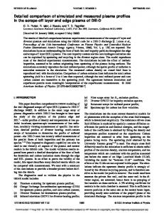
FIG. 1. 共a兲 Sketch of a typical plasma structure with intermediate DL found in experiments. 共b兲 Typical, axial profile of the electric potential and its effect on the four plasma species. 共c兲 Spherical model of the plasma structure used in this paper.

plasma configuration around a contactor is even harder, because of the nonplanar geometry, more inhomogeneous plasma profiles, and the need to simulate the ambient, undisturbed plasma. Marshall and Neubauer10 tried this problem and only obtained solutions with strong fluctuations and no DL. Hubbard and Joyce11 have pointed out that the problems in the simulations come mainly from the boundary condi-

V. Lapuerta and E. Ahedo

tions, which 共i兲 are not periodical, 共ii兲 must preserve the global electrical neutrality, and 共iii兲 must simulate two counterstreaming flows and the injection of particles of the confined species. The consequence is that the dynamic behavior is affected by undesirable wave reflections at the boundaries and artificial coupling between plasma conditions at both electrodes. In view of the difficulties encountered by numerical simulations to reproduce a fully nonlinear, time-dependent solution, this paper proposes an analytical approach of the contactor problem based in a time-dependent, linear perturbation of a well-defined steady solution. This perturbation model will clarify fundamental aspects of the dynamic response, like 共i兲 the temporal modes that propagate in the multispecies plasmas at both DL sides, 共ii兲 the boundary conditions at the contactor surface and at the ambient plasma, 共iii兲 the transition and jump conditions at the mobile DL, and 共iv兲 the instability types that may develop in the global structure. The understanding of these points is an adequate basis for a consistent formulation of a steady, weakly turbulent model and for a correct design of numerical simulations. For the dynamic model to be investigated analytically we consider a simplified formulation, consisting of macroscopic plasma equations and a spherical geometry, Fig. 1共c兲. A fully macroscopic, dynamic version of the 共partially kinetic兲 model of Ahedo, Sanmartıń, and Martıńez-Sańchez12 is used. This model determines completely the parameters and spatial profiles of the steady solution 共including the transition conditions to the DL兲, which is essential to apply consistently the perturbation techniques. The model of Ahedo et al. neglects collisions with neutrals in the plasma plume. A later model of Ahedo,13 which includes external ionization due to electron–neutral collisions, could not be used here because a fully macroscopic formulation of it is not completed yet. For a spatially nonuniform solution, the temporal perturbation theory determines the spatial profile for each individual mode of 共complex兲 frequency ⍀. The analysis here will contemplate both the response to a time-dependent plasma emission and the 共absolute兲 instability behavior of the steady solution, excepting kinetic 共or micro-兲 instabilities that cannot be analyzed with a macroscopic model. Due to the dissimilar characteristic times of response of ions and electrons, there are, at least, two distinguished ranges of frequencies, with rather different plasma dynamics. In this paper, the discussion is restricted to low-frequency modes, dominated by ion dynamics. The paper is organized as follows. Section II details the hypotheses and equations that constitute the time-dependent model, and analyzes the quasisteady equations of a thin, free DL. Section III briefly summarizes the parameters and conditions that define the steady presheath/DL/core solution. Section IV formulates the perturbation model, with special attention to conditions at the DL. Section V completes the details of the perturbation model in each region and defines the procedure for the numerical integration; an asymptotic solution for large ion frequencies is presented, also. Section VI has two subsections: The first one studies the regular plasma response to a time-dependent plasma emission; and



Dynamic model of a plasma structure with an . . .

the second one discusses the nonexistence of a radial, ion– electron macroinstability, in particular of the Buneman instability. Section VII collects final comments and extensions of the present work. II. FORMULATION OF THE MODEL

A spherically symmetric model is considered with r and t as the radial and temporal variables. The contactor is a sphere of radius R which emits an artificial plasma into a quiescent, unmagnetized plasma, Fig. 1共c兲. The undisturbed density and temperature of the ambient plasma are N ⬁ and T ⬁ , respectively. The contactor is biased to a potential ⌽(R,t) positive and large compared to the mean plasma temperature. Hence, ions from the ambient plasma 共species a兲 are prevented from approaching the contactor, while ambient electrons 共species e兲 are accelerated inwards and, part of them, collected by the contactor; let I e (t) be the electron current collected by the contactor. The artificial plasma is characterized by the current I i (t) of emitted ions 共species i兲, which are accelerated outwards, and by the equilibrium temperature T c of emitted electrons 共species c兲, which remain confined around the contactor. The emitted current I i (t) is assumed large enough to sustain a plasma structure consisting of 共i兲 a quasineutral plasma cloud 共the core兲 surrounding the contactor, 共ii兲 a space-charge double layer, where most of the potential drop takes place, and 共iii兲 an exterior quasineutral region 共the presheath兲. The ratio ␭ D⬁ /R, with ␭ D⬁ ⫽( ⑀ 0 T e /e 2 N ⬁ ) 1/2, is considered small enough to adopt a two-scale analysis, where the DL is treated as a free discontinuity in the quasineutral scale 共related to R兲. The thickness ⌬r D of a quasiplanar, strong DL verifies5 ⌬r D ⬃␭ D⬁ 共 e⌬⌽ D /T ⬁ 兲 3/4Ⰶr D , ⫺ ⌬⌽ D ⫽⌽(r D )

where r⫽r D (t) is the DL position and ⫹ ) is the potential jump across the DL. The plasma/ ⫺⌽(r D ⫺ ,t), contactor model must determine I e (t), r D (t), ⌽(r D ⫹ ⌽(r D ,t), and the plasma profiles in terms of ⌽(R,t), I i (t), and the rest of plasma parameters. The dynamic model developed here considers the plasma response to small, dynamic perturbations of the steady solution, in particular those produced by an unsteady plasma emission, I i 共 t 兲 ⫽I i0 ⫹I i1 共 t 兲 , I i1 ⰆI i0 . The dynamic response is obtained as sum of the steady solution and the dynamic solution of the linear perturbation problem; subscripts 0 and 1 are used throughout the paper for these two solutions, respectively. The dynamics of the four plasma species is represented by the following macroscopic equations:

⳵N␣ ⳵ ⫹ 共 N ␣ V ␣ 兲 ⫽0, ⳵t ⳵r m␣

⳵V␣ ⳵V␣ ⳵⌽ 1 ⳵ N ␣T ␣ ⫹m ␣ V ␣ ⫹ ⫹q ␣ ⫽0, ⳵t ⳵r N␣ ⳵r ⳵r 1⫺% ␣

T ␣N ␣

共1兲

⫽const,

where ␣ ⫽i,e,a,c is representing each species, V ␣ are macroscopic velocities, N ␣ are densities, T ␣ are temperatures,

2695

m ␣ are particle masses, q ␣ ⫽⫾e are electric charges 共and all ions are assumed singly charged兲, and % ␣ are heat specific ratios 共equal to three for free species i and e, and one for confined species, a and c, according to Ref. 12兲. Collisions among the different plasma species and with neutrals are not included in this model. Poisson equation for the electrostatic potential

冉冊

␧0 ⳵ 2 ⳵⌽ r ⫽⫺ ⳵r r2 ⳵r

兺␣ q ␣ N ␣ ,

共2兲

closes the set of Eq. 共1兲; it simplifies to the quasineutral condition 兺 q ␣ N ␣ ⯝0, in core and presheath. These two regions are matched through the jump conditions across the DL discontinuity, which are obtained from the DL internal equations. A. Quasisteady model of the double layer

Plasma equations inside a quasiplanar DL admit a simple formulation. First, in a reference frame tied to the DL, the plasma motion is quasisteady 共except for very large frequency modes, not considered in this paper兲 and verifies N ␣ ˜V ␣ ⯝const,

共3兲

m ␣ ˜V ␣2 /2⫹H ␣ ⫹q ␣ ⌽⯝const,

where ˜V ␣ ⫽V ␣ ⫺dr D /dt are velocities in the DL frame, H ␣ ⫽% ␣ T ␣ /(% ␣ ⫺1)⫹const, for free species, and H ␣ ⫽T ␣ ln N␣⫹const, for confined species. Second, Eq. 共2兲 simplifies to its quasiplanar form, which, using Eq. 共3兲, yields the integral law

冉冊

␧ 0 d⌽ 2 dr

2

⫺S 共 ⌽ 兲 ⯝const, S⫽

兺␣ 共 m ␣ N ␣ ˜V ␣2 ⫹N ␣ T ␣ 兲 .

共4兲

This is the equation of conservation of momentum of the whole plasma, and states the equilibrium between the pressure of the electric field and the stagnation pressure of the plasma; S(⌽) is normally termed the Sagdeev potential. Constants in Eqs. 共3兲 and 共4兲 are determined from the matching between the two quasineutral regions and the DL. The ratio between the electric fields outside and inside the DL is ␭ D⬁ /r D Ⰶ1, so this two-scale analysis may consider ⫺ ⫹ . Then, the constant of and r D that ␭ D⬁ d(ln ⌽)/dr→0 at r D Eq. 共4兲 is ⫹ ⫺ S共 ⌽D 兲 ⫽S 共 ⌽ D 兲.

共5兲

This equality is also the expression of Langmuir condition, which states both that the plasma pressure at both DL sides is the same, and the total electric charge of the DL is zero. More generally, the Sagdeev potential inside the DL must satisfy ⫺ ⫹ S 共 ⌽ 兲 ⫺S 共 ⌽ D 兲 ⫽S 共 ⌽ 兲 ⫺S 共 ⌽ D 兲 ⬎0.

共6兲

Then, from Taylor expansion of the left-hand sides of Eq. ⫾ ⫾ )⫽⫺ 兺 q ␣ N ␣ (⌽ D )⫽0, a transition 共6兲, and since S ⬘ (⌽ D from a quasineutral plasma to a DL requires that ⫾ ⫾ ⫾ S ⬙共 ⌽ D 兲 ⬎0, or 关 S ⬙ 共 ⌽ D 兲 ⫽0 and S ⵮ 共 ⌽ D 兲 ⫽0 兴 ,

共7兲


2696



which are the regular and singular forms, respectively, of Bohm condition. Once constants in Eqs. 共3兲 and 共4兲 are set, plasma profiles inside the DL are obtained by integrating Eq. 共4兲. This integration is straightforward when S(⌽) is a one-branch function. Furthermore, only Langmuir and Bohm conditions are then needed to solve the response of the quasineutral plasma.

r 2 N e0 V e0 ⫽const⫽J e0 ,

共8兲

2 /2⫺e⌽ 0 ⫹3T e0 /2⫽3T ⬁ /2, m e V e0

共9兲

2 /N ⬁2 , T e0 /T ⬁ ⫽N e0

共10兲

r 2 N i0 V i0 ⫽const⫽J i0 ,

共11兲

2 /2⫹e⌽ 0 ⫹3T i0 /2⫽const⫽K i0R , m i V i0

共12兲

2 2 /N i0R , T i0 /T i0R ⫽N i0

共13兲

N a0 ⫽N ⬁ exp共 ⫺e⌽ 0 /T ⬁ 兲 , r⬎r D0 ,

共14兲

冉

冊

⌽ 0 ⫺⌽ 0R , r⬍r D0 , T c0

共15兲

where: Subscript R refers to r⫽R; J e0 (⬍0) and J i0 are the particle flows of the two free species; and the restriction of each confined species to just one side of the strong DL is consistent with the macroscopic model and simplifies the treatment of the quasineutral model. In the core and presheath, the quasineutral condition N i0 ⫹N a0 ⫺N e0 ⫺N c0 ⯝0,

共16兲

is added to close the problem. Equations 共8兲–共16兲 define implicitly the spatial profiles of ⌽ 0 (r) and the rest of the plasma variables. For the desired range of parameters this solution presents turning points with d/dr⫽⫾⬁, which must denote either a transition to a space-charge layer or the contactor surface. For instance, the electric field verifies d⌽ 0 2 Q 0 ⫽ , dr r P0 Q 0 ⫽⫺

兺␣

P 0⫽

共 m ␣ N ␣ 0 V ␣2 0 ⫹N ␣ 0 T ␣ 0 兲

␣

A brief derivation of the steady solution of Ahedo et al. is presented here, with emphasis on the aspects that are relevant for the perturbation problem, like transitions to the DL, boundary conditions at the contactor, and dimensionless parameters that define the response. Subjects like the uniqueness of the solution and the orbital-motion-limit regime, are omitted. For steady boundary conditions, the steady solution 共denoted with subscript 0兲 verifies the set of conservation equations

兺␣ %

q ␣2 N ␣ 0 2 ␣ T ␣ 0 ⫺m ␣ V ␣ 0

q ␣ N ␣ 0 m ␣ V ␣2 0 , % ␣ T ␣ 0 ⫺m ␣ V ␣2 0

共18兲

It is easily seen that P 0 is the second derivative of Sagdeev potential, S 0⬙ , so Eq. 共18兲 is the Bohm singular condition. ⫹ , from presheath to DL is one of The transition point, r⫽r D0 the solutions of this equation 关no valid solution of the DL has ⫹ )⬎0兴. The DL–core transition point, been found with P 0 (r D0 ⫺ r⫽r D0 , is obtained from Langmuir condition 共5兲, which here takes the form

冋兺

III. STEADY SOLUTION

N c0 ⫽N c0R exp e

P 0 ⫽0.

册

⫹

r D0 ⫺ r D0

⫽0.

⫹ , the transition from DL to It comes out that, contrary to r D0 ⫺ )⬎0, so a regular solution core is a regular point with P 0 (r D0 ⫺ . Since, in the core requires P 0 to be positive for R⬍r⬍r D0 in a loose sense, condition P 0 ⫽0 is related to ‘‘sonic’’ conditions of the emitted plasma,12 P 0 (R)⫽0 will be imposed unless stated otherwise. This eliminates the ion velocity at the contactor exhaust, V i0R , as a free parameter. Also, it was justified by Ahedo et al. that, since the emitted ions flow sonic/supersonically, T i0 affects the solution weakly and can be neglected. With respect to the formulation presented here the model discussed in Ref. 12 makes two additional hypotheses that restrict the parametric range of validity of the solution. First, it disregards thermal effects of the attracted electrons in the core, which is valid while the core size is not very large. Second, it neglects the influence of the emitted ions in the presheath solution, which is valid for large contactor potentials (e⌽ 0R /T ⬁ ⬎102 , roughly兲. The two restrictions will be kept here; only the second one may have some influence on the low-frequency response, as will be commented later. For a compact representation of the solution, R, N ⬁ , and T ⬁ are used to define nondimensional variables and parameters:

␰⫽

r e⌽ T␣ N␣ , t ␣⫽ , n ␣⫽ , , ␾⫽ R T⬁ T⬁ N⬁

v ␣⫽

V␣ 共 T ⬁ /m ␣ 兲

1/2

, j ␣⫽

J␣ R N ⬁ 共 T ⬁ /m ␣ 兲 1/2 2

.

Using this nondimensionalization, the steady solution depends on three parameters; in particular, the C-V characteristic takes the form j e0 ⫽ j e0 ( j i0 , ␾ 0R ,t c0 ). Figure 2 shows examples of the C-V response and steady plasma profiles. IV. PERTURBATION MODEL

A generic variable or parameter, let us say f, is decomposed as f 共 r,t 兲 ⯝ f 0 共 r 兲 ⫹ f 1 共 r,t 兲 ,

, 共17兲

so turning 共singular兲 points of the quasineutral solution correspond to

f 1 共 r,t 兲 ⫽ 共 2 ␲ 兲

⫺1

冕

L

共19兲 f 1 共 r,⍀ 兲 exp共 ⫺i⍀t 兲 d⍀,

where f 0 (r) is the steady part, f 1 (r,t) is the time-dependent perturbation, f 1 (r,⍀) is its Laplace transform, ⍀⫽⍀ re ⫹i⍀ im is a complex frequency and L is the Laplace integra-




2697

N ␣ 1 K ␣ 1 ⫺q ␣ ⌽ 1 ⫺m ␣ V ␣2 0 J ␣ 1 /J ␣ 0 ⫽ , N ␣0 % ␣ T ␣ 0 ⫺m ␣ V ␣2 0

共22兲

V ␣ 1 ⫺K ␣ 1 ⫹q ␣ ⌽ 1 ⫺% ␣ T ␣ 0 J ␣ 1 /J ␣ 0 ⫽ , V ␣0 % ␣ T ␣ 0 ⫺m ␣ V ␣2 0

obtained from 共20兲. In the core and presheath, these equations are completed with 兺 q ␣ N ␣ 1 ⯝0. Substituting here N ␣ 1 from Eq. 共22兲, the perturbed electric potential ⌽ 1 is obtained as a linear combination of J ␣ 1 and K ␣ 1 Q1 ⌽ 1⫽ , Q 1⫽ P0

兺␣ q ␣ N ␣ 0

K ␣ 1 ⫺m ␣ V ␣2 0 J ␣ 1 /J ␣ 0 % ␣ T ␣ 0 ⫺m ␣ V ␣2 0

,

共23兲

with P 0 defined in Eq. 共17兲. Equations 共21兲–共23兲 form a closed set for the two quasineutral regions. Plasma perturbations produce a displacement, r D1 (t) ⫽r D (t)⫺r D0 , of the free DL from its position in the steady solution, which must be determined. Because of this displacement and in order to represent the dynamic response 共zeroth plus first-order solutions兲 the spatial variable r needs to be stretched with the linear change r→s(r,t)

再

r D0 ⫺R , for r⬍r D s⫺r D0 r ⫽ D 共 t 兲 ⫺R , r⫺r D 共 t 兲 1, for r⬎r D

FIG. 2. Steady solution: 共a兲 Current-voltage response, j e0 ( j i0 , ␾ 0R ), for t c0 ⫽10; the dashed line corresponds to ␰ D0 ⫽1, the transition to the no-core solution. 共b兲 and 共c兲 Spatial profile of the electric potential and the densities ⫹ of the two free species for ␾ 0R ⫽10, j i0 ⫽14.3, and t c0 ⫽1; ␰ ⫽ ␰ D0 and ␰ ⫽1 are singular points of the quasineutral equations; n i0 ⫺n e0 is equal to n c0 in the core and to ⫺n a0 in the presheath.

tion path. Modes are purely oscillatory 共in time兲 when ⍀ is real, and purely monotonic when i⍀ is real. The designation of ‘‘acoustic’’ and ‘‘standing’’ modes, natural for ⍀ real, will be employed here for any ⍀, whether real or complex. To facilitate the mathematical treatment of the perturbation equations, the perturbed particle flow and mechanical energy, J ␣ 1 ⫽r 2 共 N ␣ 1 V ␣ 0 ⫹N ␣ 0 V ␣ 1 兲 , K ␣ 1 ⫽m ␣ V ␣ 0 V ␣ 1 ⫹% ␣ T ␣ 0 N ␣ 1 /N ␣ 0 ⫹q ␣ ⌽ 1 ,

共20兲

respectively, will be used as perturbation variables, instead of N ␣ 1 and V ␣ 1 . Applying expansion 共19兲 to Eq. 共1兲, the perturbation equations for each plasma species and each ⍀-mode are dJ ␣ 1 /dr⫺i⍀r 2 N ␣ 1 ⫽0, dK ␣ 1 /dr⫺i⍀m ␣ V ␣ 1 ⫽0, with

共21兲

共24兲

which transforms r⫽R and r⫽r D (t) into s⫽R and s ⫽r D0 , respectively. Once solutions f 0 (r) and f 1 (r,t) are known, the total response of f at s⫽s * and any t is 共neglecting nonlinear contributions兲 f 共 r 共 s * ,t 兲 ,t 兲 ⯝ f 0 共 s * 兲 ⫹ ˆf 1 共 s * ,t 兲 , ˆf 1 共 s * ,t 兲 ⫽ f 1 共 s * ,t 兲 ⫹ 关 r 共 s * ,t 兲 ⫺s * 兴

df0 共 s*兲. dr

In particular, the total perturbation at each DL side is ⫾ ˆf 1 (r D0 ,t), and the DL jump conditions of the perturbation problem, derived from Eqs. 共3兲 and 共4兲, are r

⫹

2 N ␣ 0 兴 ⫺D0 ⫽0, 关 J ␣ 1 ⫹i⍀r D1 r D0 r D0

r

⫹

D0 ⫽0, 关 K ␣ 1 ⫹i⍀r D1 m ␣ V ␣ 0 兴 r ⫺

兺␣

冋

共25兲

D0

2m ␣ N ␣ 0 V ␣ 0 共 V ␣ 1 ⫹i⍀r D1 兲 ⫹m ␣ N ␣ 1 V ␣2 0 ⫹% ␣ N ␣ 1 T ␣ 0

d ⫹r D1 共 m ␣ N ␣ 0 V ␣2 0 ⫹N ␣ 0 T ␣ 0 兲 dr

册

⫹

r D0 ⫺ r D0

⫽0,

where the Laplace transform and zeroth-order jump conditions have already been applied, and i⍀r D1 is the displacement velocity of the DL. The last equation is the perturbation of the Langmuir condition. The temporal response of ions and electrons is very different due to their dissimilar masses. Then, there are, at least, two distinguished ranges for the frequency of the perturbation modes: Ion frequencies, ⍀⬃R ⫺1 冑T ⬁ /m i , when the


2698



electron response is quasisteady, and plasma dynamics are based in ion–electron modes; and electron frequencies, ⍀ ⬃R ⫺1 冑T ⬁ /m e , when ions stay rigid in their stationary response, and plasma dynamics are dominated by electron– electron modes and, perhaps, space-charge modes. Each frequency range has its own set of equations and boundary conditions, if variables are nondimensionalized adequately. For modes in the ion frequency range, the convenient dimensionless frequency is

␻ ⫽⍀R/ 冑T ⬁ /m i , with ␻ ⫽O(1) as the distinguished case, and the temporal derivatives are eliminated from electron equations when the asymptotic limit m e /m i →0 is taken. Boundary conditions of the perturbation problem in the core and presheath consists of: 共i兲 No perturbations of the ambient plasma at r⫽⬁; 共ii兲 the dynamic solution is bounded at any point; 共iii兲 jump condition 共25兲 at the DL are satisfied; 共iv兲 perturbations on conditions at the contactor exhaust are specified. For ion frequency modes, the perturbation of the plasma emission, J i1 (R,t)⫽I i1 (t)/4␲ e, is the most relevant one. V. INTEGRATION OF THE PERTURBATION PROBLEM

Like the zeroth-order problem, the perturbation equations are integrated from ␰ ⫽⬁ to ␰ ⫽1. The presheath problem, for a steady solution with n i Ⰶn e , consists of relations n a1 ⯝n e1 , j e1 ⫽const, k e1 ⫽0, 2 2 j e1 / j e0 ⫺ 共 v e0 ⫺3t e0 兲 k a1 q 1 v e0 ␾ 1⫽ ⫽ , 2 p0 1⫹3t e0 ⫺ v e0

共26兲

and two differential equations for the dynamics of ambient ions 2 k a1 ⫺ v e0 j e1 / j e0 1 d j a1 ⫺i␻ a n e0 ⫽0, 2 2 d␰ ␰ 1⫹3t e0 ⫺ v e0

j a1 dk a1 ⫺i␻ a 2 ⫽0. d␰ ␰ n e0

共27兲

In Eqs. 共26兲 and 共27兲: k ␣ 1 , p 0 , and q 1 are the dimensionless counterparts of their corresponding capital case variable, Eqs. 共20兲–共23兲; ␻ a ⫽ ␻ 冑m a /m i is used for convenience when ambient and emitted ions are different; and zero perturbation of the ambient plasma at r⫽⬁ has been assumed. Notice that j e1 ⫽0 is compatible with n e1 ⫽ v e1 ⫽0 at r ⫽⬁. The general solution of Eq. 共27兲 is a linear combination of three modes, and boundary conditions are imposed at ␰ ⫹ ⫽⬁ and ␰ ⫽ ␰ D0 . Taking into account the temporal dependence: exp(⫺i⍀t), the asymptotic behavior for ␻ a ␰ D0 Ⰷ1 共see next Subsection for a detailed derivation兲 shows that there are one quasisteady mode, proportional to j e1 , and two ion–acoustic modes. Disregarding the acoustic mode that travel inwards 共when ␻ re⫽0) and is unbounded at ␰ ⫽⬁ 共when ␻ im⫽0), the asymptotic solution of Eq. 共27兲 at ␰ Ⰷ ␰ D0 , 兩 ␻ a 兩 ⫺1/5 is

j a1 共 ␰ 兲 ⯝ j e1

冋

2 4ij e0

␻ a␰

5

册冋冉冊册

⫹••• ⫹a ⬁

1 i␻ a exp ␰ ⫹••• . 2␰ 2

共28兲

Next, two conditions are imposed at the presheath/DL boundary. First, the DL is a barrier for the ambient ions, so their relative velocity there is zero, ⫹ ␰ ⫽ ␰ D0 :

j a1 / ␰ 2 n e0 ⫹i␻ a ␰ D1 ⫽0.

共29兲

⫹ ⫹ is a singular point with p 0 ( ␰ D0 )⫽0, the Second, since ␰ D0 solution must be bounded there. From the expression for the electric potential one has

␾ˆ 1 ⫽ 共 q 1 ⫹2q 0 ␰ D1 / ␰ D0 兲 /p 0 , 共with q 0 ⬅Q 0 /eN ⬁ ), so the numerator in the right-hand side ⫹ . Substituting q 0 and q 1 , this condimust be zero at ␰ ⫽ ␰ D0 tion becomes ⫹ ␰ ⫽ ␰ D0 :

2 v e0 共 j e1 / j e0 ⫺2 ␰ D1 / ␰ D0 兲 ⫺k a1 ⫽0.

共30兲

It can be shown that Eq. 共30兲 is equivalent to the Bohm ⫹ ) singular condition 共7兲 of the perturbation problem: Sˆ 1⬙ (r D0 ⫽0. Conditions 共28兲–共30兲 include three parameters: ␰ D1 , j e1 , and a ⬁ . Thus, for each ␻ , the integration of Eqs. 共26兲 and 共27兲 yields two relations between these parameters. Therefore, the perturbation solution in the presheath is universal and proportional to one parameter; the most convenient one is j e1 . The numerical integration of the presheath equations presents two problems. The first one is the singularity at ␰ ⫹ ⫽ ␰ D0 . The change of independent variable ␰ → 兰 d ␰ / p 0 makes the equations regular and the numerical integration straightforward. The second problem is harder to solve. In principle, to avoid the unbounded 共or out-traveling兲 mode at ␰ ⫽⬁, the integration should proceed from ␰ ⫽⬁ with the two independent modes of the asymptotic solution 共28兲 as ‘‘initial’’ conditions. However, their different growth scale makes this procedure impracticable. We were thus forced to ⫹ and to use an iterative scheme to integrate from ␰ ⫽ ␰ D0 match with the asymptotic solution at ␰ Ⰷ ␰ D0 . The numeri⫹ with conditions 共29兲 and 共30兲 yields cal integration from ␰ D0 a solution that is the combination of two independent modes, each one proportional to j e1 and ␰ D1 . The correct matching with the asymptotic solution must provide the correct value of j e1 / ␰ D1 . In each iteration step, the solution is built up with two independent modes, each one with a ratio ␰ D1 / j e1 close to a predetermined value. This numerical solution is stopped before the explosive modes develop, at ␰ ⫽ ␰ say, * and is matched there to the asymptotic solution. This determines the value of ␰ D1 / j e1 to be used in the next iteration step. As the values of ␰ D1 / j e1 are closer to the correct one, the numerical solution can proceed farther. The iteration finishes when the matching point ␰ is within the admissible * interval of the asymptotic solution. The core problem for species e, c, and i consists of the quasisteady equations for electrons ⫹ j e1 ⫽ j e1 共 ␰ D0 兲 , k e1 ⫽0, j c1 ⫽0, k c1 ⫽0,

共31兲

a quasineutral equation for the electric potential




2 2 ␾ 1 ⫽q 1 /p 0 , p 0 ⫽n c0 /t c0 ⫺n i0 / v i0 ⫺n e0 / v e0 , 2 q 1 ⫽n i0 共 j i1 / j i0 ⫺k i1 / v i0 兲 ⫺n e0 j e1 / j e0 ,

共32兲

and the dynamic equations for ions

冉

冊

d j i1 i␻ k i1 ⫺ ␾ 1 ⫺ j i1 ⫺ j i0 ⫽0, 2 d␰ v i0 v i0 共33兲

dk i1 i␻ ⫺ 共 k ⫺ ␾ 1 兲 ⫽0. d␰ v i0 i1

Once ␾ 1 is substituted, the general solution of Eq. 共33兲, is combination of two ion–acoustic modes 共which are the solution of the homogeneous problem兲 and a standing mode, proportional to j e1 . Four boundary conditions have already been imposed in Eq. 共31兲 for the quasisteady electrons: j e1 and k e1 are constant across the DL; zero flow of species c across the DL; n c1 and ␾ 1 verify the Boltzmann equilibrium equation. Three boundary conditions are still needed to close the problem. The first one is the Langmuir condition 共4兲, which, with the help of the rest of DL jump conditions, becomes ⫺ ⫹ ⫺ v i0D 兲共 v i0D

冉

⫺ j i1D

j i0

⫹

⫺ ⫹ ⫽ 共 v e0D ⫺2 v e0D 兲

i␻␰ D1 ⫺ v i0D

⫺

冉

⫺ ⫺ ⫹i␻␰ D1 v i0D 2 ␰ D1 k i1D ⫺ ⫹ ⫺ ␰ D0 v i0D v i0D

冊

j e0 j e1 2 ␰ D1 ⫺ , j i0 j e0 ␰ D0

D 共 ␻ ; j i0 , ␾ 0R ,t c0 兲 ⬅det A⫽0.

共36兲

Unstable solutions correspond to eigenmodes with ␻ im ⬎0. A. Asymptotic analysis for 円 ␻ 円 š1

冊

共34兲

˜ ⬁ ␣ p 共 ␰ 兲 exp关 ⫺ ␤ p 共 ␰ 兲兴 ⫹ j e1 j a1 共 ␰ 兲 ⯝a

共35兲

关For p 0 (1)⬎0, j i1 (1)⫽ j i1R and k i1 (1)⫽k i1R are specified.兴 Since the core is assumed quasineutral, ␾ 1 (1) is determined from Eq. 共32兲

␾ 1 共 1 兲 ⬅ ␾ 1N ⫽ lim q 1 /p 0 . ␰ →1

If the perturbation of ␾ 1 at the contactor surface wants to be fixed, say ␾ 1R , and differs from ␾ 1N , the Appendix shows that a small space-charge layer is formed, between the contactor at the quasineutral core, to adjust both values of ␾ 1 . According to Eqs. 共21兲 and 共22兲, in the zero-Debye-length limit, j ␣ 1 and k ␣ 1 are invariant across that layer, but n ␣ 1 and v ␣ 1 change with ␾ 1 . The practical procedure to solve core equations is the following: First, the presheath solution provides ␰ D1 / j e1 ; ⫺ as linear combination of j e1 and second, Eq. 共34兲 yields k i1D ⫺ ⫺ to ␰ j i1D ; third, the integration of Eq. 共33兲 from ␰ ⫽ ␰ D0 ⫽1 yields the solution of the core in terms of these two flow parameters 关this numerical integration does not pose any difficulty once the equations are made regular around ␰ ⫽1 in a way similar to the presheath兴; and fourth, imposing the two conditions 共35兲 at ␰ ⫽1, one has ⫺ j e1 兴 A⫽ j i1R B, 关 j i1D

with A and B matrices of sizes 2⫻2 and 1⫻2, respectively, which determines completely the perturbation response in terms of j i1R and ␻ . Temporal eigenmodes of a particular steady solution 共characterized by j i0 , ␾ 0R , and t c0 ) correspond to a nonzero response to j i1R ⫽0, so they are the solutions of the global dispersion equation

Before computed results are discussed, an asymptotic solution of the perturbation response for large ion frequencies is presented. The aim of this analysis is threefold: First, to get a better understanding of the different plasma modes that are launched in the two plasma regions and their interaction; second, to obtain asymptotic scaling laws for the variation of the main plasma parameters; and third, to have an alternative integration method for 兩 ␻ 兩 Ⰷ1, when the preceding numerical scheme becomes slow and unreliable. The asymptotic solution of presheath equation 共27兲 for 兩 ␻ a ␰ D0 兩 Ⰷ1 is the combination of the WKB 共Wentzel– Kramers–Brillouin兲 solution14 of the homogeneous problem plus a particular solution proportional to j e1

with superscripts ⫹ and ⫺ naming each of the DL sides. Finally, two boundary conditions on species i are imposed at ␰ ⫽1. For p 0 (1)⫽0, one imposes the perturbation of the ion flow and the boundedness of ␾ 1 , Eq. 共32兲: j i1 共 1 兲 ⫽ j i1R , q 1 共 1 兲 ⫽0.

2699

j e0 k a1 共 ␰ 兲 ⯝⫺

4iv e0 1⫹3t e0 , 2 ␻ a ␰ 1⫹3t e0 ⫺ v e0 共37兲

ã ⬁ 2 exp关 ⫺ ␤ p 共 ␰ 兲兴 ⫹ j e1 v e0 , ␣ p共 ␰ 兲

with 2 ⫺1/4 ⫺1/2 ␣ p 共 ␰ 兲 ⫽ 共 1⫹3t e0 ⫺ v e0 兲 v e0 ,

␤ p 共 ␰ 兲 ⫽⫺i␻ a

冕

␰ ⫹

␰ D0

2 ⫺1/2 d␰, 兲共 1⫹3t e0 ⫺ v e0

and ã ⬁ a constant — proportional to a ⬁ in Eq. 共28兲. The expression of ␤ p shows that the WKB mode is an ion– electron mode traveling outwards with 共dimensionless兲 local, 2 group velocity 冑1⫹3t e0 ⫺ v e0 . ⫹ Close to ␰ D0 it is 2 ⯝a 0 共 ␰ / ␰ D0 ⫺1 兲 1/2, 1⫹3t e0 ⫺ v e0 ⫹ ⫹ 冑2( v e0D ) 2 ⫺1), so the presheath/DL with a 0 ⫽⫺2 3/2( v e0D boundary is a singular point of the WKB solution. For ␰ / ␰ D0 ⫺1Ⰶ1, the solution that matches with 共37兲 is

j a1 共 ␰ 兲 ⯝

再

ã ⬁ c 1 共 Ai共 z 兲 ⫹iBi共 z 兲兲 ⫹ j e1 c 2 Hi共 z 兲 , 共 ␻ im⫽0 兲 , ˜ ⬁ c 1 Ai共 z 兲 ⫺ j e1 c 2 Gi共 z 兲 , 共 ␻ im⫽0 兲 , 2ia

where Ai, Bi, Gi, and Hi are Airy functions,15 and z共 ␰ 兲⫽

c 1⫽

共 2 ␻ a ␰ D0 兲 2/3

a 1/3 0

冉

冑␲ 共 2 ␻ a ␰ D0 兲 1/6 ⫹ 1/2 兩 v e0D 兩 1/2a 1/3 0 i

␰ ␰ D0

⫺1

, c 2⫽

冊

1/2

,

⫹ 8 ␲ i共 v e0D 兲3 1/3 a 4/3 0 共 2 ␻ a ␰ D0 兲

;


2700



the expressions for k a1 ( ␰ ) are omitted. Boundary conditions ⫹ relate ã ⬁ and j e1 to ␰ D1 . Keeping 共29兲 and 共30兲 at ␰ ⫽ ␰ D0 only the dominant terms, one has j e1 冑3 共 2a 0 ␻ a ␰ D0 兲 4/3 ␰ D1 ⯝ , ⫹ j e0 8 ␲ 4Ai共 0 兲共 v e0D 兲 4 ␰ D0 共38兲

ã ⬁ i共 2 ␻ a ␰ D0 兲 5/6a 1/3 ␰ D1 0 ⯝c 3 , ⫹ 1/2 ␰ j e0 D0 8Ai共 0 兲兩 ␲ v e0D 兩

with c 3 equal to 1 and 2i1/2, for ␻ im ⫽0 and ␻ im ⫽0, respectively. In the core, the asymptotic solution of Eq. 共33兲, for 兩 ␻ 兩 Ⰷ1, is the combination of two WKB modes plus the particular solution proportional to j e1 j i1 共 ␰ 兲 ⫽ ␣ 关 C ⫹ exp共 ⫺ ␤ ⫹ 兲 ⫹C ⫺ exp共 ⫺ ␤ ⫺ 兲兴 ⫹O 共 j e1 ␻ ⫺1 兲 , k i1 共 ␰ 兲 ⫽

1 关 C exp共 ⫺ ␤ ⫹ 兲 ⫺C ⫺ exp共 ⫺ ␤ ⫺ 兲兴 j i0 ␣ ⫹ ⫺

with

␣共 ␰ 兲⫽

n e0 2 n c0 /t c0 ⫺n e0 / v e0

冋冉 1

2 n i0 v i0

␤ ⫾ 共 ␰ 兲 ⫽⫺i␻

冕

n c0 n e0 ⫺ 2 t c0 v e0

冊册

共39兲

j e1 , j e0

1/4

FIG. 3. Evolution of the electric potential for two oscillatory perturbations on the plasma emission: 共a兲 ␻ ⫽1.5, j i1R / j i0 ⫽0.2, j i0 ⫽9.1, ␾ 0R ⫽10, and t c0 ⫽1; 共b兲 ␻ ⫽3, j i1R / j i0 ⫽0.2, j i0 ⫽164.6, ␾ 0R ⫽10, and t c0 ⫽1. The displacement of the DL in 共b兲 is imperceptible: r D1 /r D0 ⬍0.15%.

,

␰

d␰

1

2 兲兴 1/2 v i0 ⫾ 关共 t c0 n i0 兲 / 共 n c0 ⫺n e0 t c0 / v e0

.

The expression for ␤ ⫾ says that the two WKB modes are mounted on the out-streaming ion beam and travel in opposite directions with a sound speed that depends weakly on v e0 . Imposing boundary condition 共35兲 at ␰ ⫽1, one has C ⫺ ⫽0,

2 C ⫹ ⫽ v i0R j i1R ,

so there is no mode traveling inwards from the ion beam. 关For p 0 (1)⬎0, both ion–acoustic modes are generally present.兴 Finally, the relation between j e1 and j i1R is obtained from Langmuir condition 共34兲; for 兩 ␻ 兩 Ⰷ1 this reduces to ⫺ ⫹ ⫺ ⫺ / v i0D ⫺i␻␰ D1 j i0 / v i0D ⫹o 共 ␻␰ D1 兲 ⯝ j i1D . j e1 v e0D

共40兲

VI. RESULTS A. Dynamic response to perturbations in plasma emission

Figure 3 shows the spatial-temporal response of the electric potential, ⌽(r,t)⫽⌽ 0 (r)⫹⌽ 1 (r,t), for two different oscillation modes on J i (R,t). Nonlinear perturbation terms are not included, so large perturbations in the plots are intended only to stand out the salient features of the plasma response. The precedent analysis has shown that a perturbation J i1R is transmitted along the core by an outward, acoustic mode mounted on the beam of emitted ions. Its 共local兲 group velocity in the laboratory frame is

V i0 ⫹

冋冉

T c0 1⫹N e0 /N c0 2 m i 1⫺ 共 N e0 /N c0 兲共 T c0 /m e V e0 兲

冊册

1/2

共41兲

and the dependence on e-beam parameters indicates that the three species are interacting. When this ion–electron mode reaches the DL, it perturbs the pressure balance at the DL, which results in a perturbation of the flow of incoming electrons and a DL displacement, according to Langmuir and 共singular兲 Bohm conditions. The perturbation on J e1 is transmitted as a standing mode to both core and presheath. The DL displacement r D1 excites another acoustic mode on the ambient ions that travels outwards with 共local兲 group veloc2 ity 冑(T ⬁ ⫹3T e0 )/m a ⫺V e0 . 关The first, ion–acoustic mode, created at the contactor surface also travels through the presheath, but it is weak there, for the parametric range we are considering. For a supersonic ion emission, P 0 (R)⬎0, one more ion–acoustic mode exists in the core.兴 The two plots of Fig. 3 illustrate that the acoustic modes dominate over the standing one as the frequency increases, and the displacement of the DL is smaller as the frequency and the core size increase. The discontinuity observed in Fig. 3 at r⫽R is the small space-charge layer that adjusts the dynamic response of ⌽ at the inner boundary of the quasineutral core, r⫽R ⫹ say, to a given value at the contactor surface, r⫽R. The physical relevance of that layer is uncertain since the transition from the internal 共keeper and hollow cathode兲 regions of the contactor




2701

FIG. 4. Evolution of the electric potential for a monotonic plasma emission: ␻ ⫽0.4i, ␾ 0R ⫽4, j i0 ⫽12.3, and t c0 ⫽1.

to the external ones has not been modeled; furthermore, whether the current or the potential bias can be externally fixed depends on the characteristics of the whole electrical circuit. Figure 4 shows the effect of a monotonic perturbation ( ␻ re⫽0, ␻ im ⬎0) on J i (R,t) for the same steady solution that Fig. 3. A response with acoustic delay substitutes here the above wave-like behavior. Otherwise, the interactions among the different species and regions are similar. The re⫹ , treat of the DL produces a small potential well at r⫽r D0 not clearly seen in Fig. 4. Figure 5共a兲 shows the temporal envelope 关the dependence on exp(⫺i⍀t) is omitted兴 of the spatial perturbation on ␾ˆ 1 for j i1R ⫽0 and different 共real兲 frequencies. Figures 5共b兲 and 5共c兲 depict the evolution of parameters j e1 and ␰ D1 with the oscillation frequency. For ␻ Ⰷ1, these plots agree with the asymptotic laws obtained from Eqs. 共38兲–共40兲

␰ D1 / ␰ D0 ⬃ 共 ␻ a ␰ D0 兲 ⫺4/3 j e1 / j e0 ,

共42兲

⫺ 2 ⫺ 兩 j i1D 兩 ⯝ 兩 j i1R 兩 v i0R ␣ 共 ␰ D0 兲,

共43兲

⫺ 兩 j e1 兩 ⯝ 兩 j i1D 兩.

共44兲

Equation 共42兲 is Bohm condition at the presheath/DL boundary. The strong decay of the relative DL displacement at high frequencies is due to the rigidity of the ambient ions in the presheath side, which constrains the DL mobility. This also explains the quasisteady form of Langmuir condition 共44兲. The decay of j i1 from the contactor surface to the DL, Eq. 共43兲, is due to the inhomogeneity of the steady spatial profile. Figure 6 is similar to Fig. 5 but for purely monotonic modes. The main novelty here is that the region affected by the perturbation of j i1R decreases with ␻ Ⰷ1 due to the acoustic delay; this makes j e1 / j i1R to decrease. For ␻ Ⰷ1 the typical thickness of the region affected by a perturbation at the contactor is ⌬r⬃⍀ ⫺1 冑T c0 /m i . Figure 7 illustrates, for oscillatory modes, the evolution of the parameters of the perturbation response with the parameters of the steady solution. We again observe that the inhomogeneity of the steady solution in the core leads to a ⫺1 , ␾ 0R , or t c0 are smaller dynamic response when ␰ D0 smaller.

FIG. 5. Response to oscillatory perturbations ( ␻ im ⫽0) on the plasma emission ( j i1R ⫽0) for ␾ 0R ⫽500, j i0 ⫽21.6, and t c0 ⫽10. 共a兲 Temporal enve˜ 1 (s) for three values of ␻ (⫽1, 5, 15). 共b兲 lope of the spatial profile of ␾ and 共c兲 Perturbation of the electron current and DL displacement, as function of the ␻ -mode; the dashed line corresponds to the WKB-type solution, valid for ␻ Ⰷ1.

B. On the radial, ion–electron instability

Numerical solving of dispersion equation 关Eq. 共36兲兴 shows that it has no solution with ␻ im ⬎0, within the range of validity of the steady solution. This result is confirmed by the asymptotic analysis for 兩 ␻ 兩 Ⰷ1: Setting j i1R ⫽0 in Eq. 共40兲 the dispersion relation becomes ⫺ ⫺ ⫹ / v i0D ⯝ij i0 ␻␰ D1 / j e1 . v e0D v i0D

This has no solution with 兩 ␻ 兩 Ⰷ1, since, from Eq. 共42兲, the right-hand side is of order ( ␻␰ D0 ) ⫺1/3. Therefore, the core/ DL/presheath structure does not present a radial, ion– electron 共macro兲instability. This conclusion refutes the analyses of Refs. 6–8, which assert the generation, in the core, of the Buneman 共macro兲instability, together with an ion–acoustic 共micro兲instability. Both are two particular cases of the ion–electron instability in a two-species plasma. However, the plasma in the core consists of three species and supports only one pair of ion– electron modes, with the ions interacting simultaneously with the two electron species, as Eq. 共41兲 shows. The local dispersion relation of the plasma 共valid for short wavelengths兲 yields that an ion–electron 共macro兲instability develops if


2702



FIG. 6. Same as Fig. 5 but for plasma emissions monotonic with time. In 共a兲 ␻ ⫽1i, 5i, 15i; in 共b兲 and 共c兲兩 ␻ 兩 ⫽ 兩 ␻ im 兩 .

2 3T e0 ⬍m e V e0 ⬍3T e0 ⫹T c0 N e0 /N c0 ,

共45兲

共for T i0 ⰆT c0 ). When N c0 ⫽0, this expression recovers the well-known instability range for a two-species plasma; but, when N e0 /N c0 ⭐O(1), the instability interval is narrow and does not include the Buneman limit. In the core, one has N e0 /N c0 ⬍1 and 兩 V e0 兩 Ⰷ 冑3T e0 /m e , typically, so there is no ion–electron macroinstability. The physical interpretation of Eq. 共45兲 is the following: c-species has a stabilizing effect 2 always, while the e-beam is de-stabilizing for m e V e0 ⬎3T e0 ; N e1 and N c1 have opposite signs in this velocity range; the combined effect of the two beams is de-stabilizing when N e1 ⬎N c1 , which justifies the upper-bound of Eq. 共45兲. For the range e⌽ 0R /T ⬁ Ⰷ1 considered here, one has N i1 /N e1 ⬃N i0 /N e0 ⬃ 冑e⌽ 0R /T ⬁ in the presheath, and the influence of the i-beam on the regular, dynamic response of the presheath is negligible. Nevertheless, the weak i-beam could still launch an ion–electron macroinstability there. The interaction of the i-beam with the ambient electrons generates two additional ion–acoustic modes in the presheath. It turns out that one of them is locally unstable, but only in the 2 ⬍T ⬁ ⫹3T e0 . region, close to the DL, where 3T e0 ⬍m e V e0 关In fact, experimentally detected fluctuations in that region4,5 could be due to this behavior.兴 We have investigated the nonlocal influence of these modes for ␻ Ⰷ1 共and e⌽ 0R /T ⬁ Ⰷ1). The two new modes were added to the asymptotic solution of the presheath, and the core/presheath coupling was appropriately modified. The resulting dispersion relation still does not detect an ion–electron 共macro兲instability. It

FIG. 7. Influence of the different steady solution parameters on the DL displacement for two perturbation modes on the plasma emission: ␻ ⫽3.16(1) and 3.16i(2). In 共a兲 ␾ 0R ⫽500 and t c0 ⫽10; in 共b兲 ␾ 0R /t c0 ⫽50 ⫺ and ␾ 0D /t c0 ⫽46; in 共c兲 t c0 ⫽10 and ␰ D0 ⫽3.98; ␰ D0 is used as independent parameter instead of j i0 .

would be interesting to analyze the case when e⌽ 0R /T ⬁ is not too large, but then the i-beam modifies also the steady solution of the presheath, a case not completed yet. The model derived here does not include collisions with the ejected gas in the plasma plume, which seem important in actual laboratory experiments. The main effect of electron–neutral collisions would be additional ionization in the core, which certainly modifies the flow and density of ions, but Ahedo13 showed that the electron beam was affected weakly. Since according to our analysis, the ion– electron instability depends on condition 共45兲 on the electron beam, it is plausible that external ionization has no significant role in the instability generation. Furthermore, if V i0 has any part on it, external ionization should have an stabilizing effect since it reduces the average ion velocity. VII. FINAL CONSIDERATIONS

We first summarize the most salient features of the preceding analysis. The dynamic response of the core/DL/ presheath structure is the combination of a quasisteady electron mode and several ion–electron modes, with different propagation characteristics in core and presheath. These two regions interact through the DL, which is itself displaced. The time-dependent behavior of the DL is determined by Langmuir law on dynamic pressure balance, Bohm law on



the plasma flow, continuity conditions on the flows of the free species, and barrier conditions on confined species. Indeed, at large frequencies ambient ions tend to be rigid, and the barrier effect restricts the DL displacement. Notice that the analysis of the time-dependent conditions at the DL is valid independently of the particular configuration of the quasineutral plasmas outside the DL; in particular it is valid for DL structures created in triple-plasma chambers. Our analytical model has also allowed a careful study of boundary conditions at the ambient plasma and the contactor surface, avoiding one of the main problems of numerical simulations. The main conclusion of the stability analysis is the nonexistence of any radial, ion–electron macroinstability of the global plasma structure, including the Buneman instability, proposed by several authors. The ion–acoustic 共micro兲instability, due to Landau kinetic effect, could not be studied with the present, macroscopic model. The classical theory9 states that the interaction of the supersonic i-beam with c-electrons generates locally unstable modes in the core. A first issue to investigate is how the presence of the e-beam modifies them: It is already known that the 共real part of the兲 phase velocity is affected. If the local modes are still unstable, the next issue would be to find the way to include them into the dynamic behavior of the global plasma structure. Two extensions of the dynamic analysis initiated here are now in progress. The first one is the investigation of the electron range of frequencies, when the plasma response is determined by electron–acoustic modes and a rigid background of ions. An unstable behavior of the plasma structure is more likely in that range, since unstable modes are detected by the local dispersion relation; the experimental data of Vannaroni et al.2 supports also this idea. The second extension is to analyze the oblique 共or nonradial兲 dynamic response, and the existence of an oblique, ion–electron instability. In a previous paper16 we already derived an oblique, stationary model, expanding spatial perturbations in the full set of spherical harmonics, but ignoring temporal perturbations, i.e., we took ⍀⫽0. The analysis of the oblique, stationary modes detected that some of them were unstable. Presumably they represent the zero-frequency limit of the oblique, ion–electron instability. ACKNOWLEDGMENTS

This research was supported by Ministerio de Educacioń y Cultura of Spain under Project PB97-0574-C04-02. APPENDIX: PERTURBATION SHEATH AT THE CONTACTOR SURFACE

Equations 共31兲–共33兲 for the core determine the value of the perturbation potential at the inner boundary of the quasineutral core,

␾ 1 共 1 ⫹ 兲 ⫽ lim q 1 /p 0 ⫽ ␾ 1N . ␰ ⫽1 ⫹


2703

If the potential at the contactor surface ␾ 1R is imposed and it differs from ␾ 1N , a boundary, space-charge layer is needed to adjust these two values. Within this layer, Eq. 共32兲 is substituted by quasiplanar Poisson equation

⑀ 2 d 2 ␾ 1 /d ␰ 2 ⫽ p 0 ␾ 1 ⫺q 1 ,

共A1兲

with ⑀ ⫽␭ D⬁ /RⰆ1. The characteristic thickness of the boundary layer depends on p 0 (1). For the regular case p 0 (1)⬎0, the expansion of p 0 and q 1 in Eq. 共A1兲 yields p 0 ␾ 1 ⫺q 1 ⫽ p 0 共 1 兲共 ␾ 1 ⫺ ␾ 1N 兲 ⫹O共 ␰ ⫺1 兲 , where we took into account that j i1 ⫽ j i1 (1)⫹O( ␰ ⫺1), k i1 ⫽k i1 (1)⫹O( ␰ ⫺1). Using ␩ ⫽ 冑p 0 (1)( ␰ ⫺1)/ ⑀ as the layer spatial variable and taking ⑀ →0, Eq. 共A1兲 becomes d 2 ␾ 1 /d ␩ 2 ⫽ ␾ 1 ⫺ ␾ 1N . The solution that verifies boundary conditions

␾ 1 兩 ␩ ⫽0 ⫽ ␾ 1R , ␾ 1 兩 ␩ ⫽⫹⬁ ⫽ ␾ 1N ,

共A2兲

is ␾ 1 ( ␩ )⯝ ␾ 1N ⫹( ␾ 1R ⫺ ␾ 1N )exp(⫺␩). For the singular case p 0 (1)⫽0, the expansion of the right-hand side of Eq. 共A1兲 is p 0 ␾ 1 ⫺q 1 ⫽a 共 ␾ 1 ⫺ ␾ 1N 兲共 ␰ ⫺1 兲 1/2⫹O共 ␰ ⫺1 兲 , with a⫽2 冑q 0 (d p 0 /d ␾ 0 ) 兩 ␰ ⫽1 , and the appropriate layer variable now is ␩ ⫽a 2/5( ␰ ⫺1)/ ⑀ 4/5, which, for ⑀ →0, transforms Eq. 共A1兲 into d 2 ␾ 1 /d ␩ 2 ⫽( ␾ 1 ⫺ ␾ 1N ) ␩ 1/2, and condition 共A2兲 still apply. The solution to this problem is

␾ 1 共 ␩ 兲 ⯝ ␾ 1N ⫹

冉冊

4 2 7/5 ␾ 1R ⫺ ␾ 1N 1/2 ␩ K 2/5 ␩ 5/4 , 2/5 ⌫ 共 2/5 兲 5 5

where ⌫(x) is the Gamma function and K 2/5 the modified Bessel function15 that satisfies K 2/5(x)⬃e ⫺x 冑␲ /2x for x Ⰷ1. Therefore, the thickness of the space-charge layer is 4/5 1/5 R ) for ⌬ ␰ ⬃ ⑀ and ⌬ ␰ ⬃ ⑀ 4/5 共i.e., ⌬r⬃␭ D⬁ and ⌬r⬃␭ D⬁ the regular and singular cases, respectively. In both situations and for ⑀ →0, j i1 and k i1 are constant in the boundary layer but not v ␣ 1 and n ␣ 1 , which depend on ␾ 1 , Eq. 共22兲. J. Williams and P. J. Wilbur, J. Spacecr. Rockets 27, 634 共1990兲. G. Vannaroni, M. Dobrowolny, E. Melchioni, F. de Venuto, and R. Giovi, J. Appl. Phys. 71, 4709 共1992兲. 3 L. Conde and L. Leoń, Phys. Plasmas 1, 2441 共1994兲. 4 N. Hershkowitz, Space Sci. Rev. 41, 351 共1985兲. 5 M. A. Raadu, Phys. Rep. 178, 26 共1989兲. 6 D. Hastings and N. Gatsonis, Acta Astron. 17, 827 共1988兲. 7 L. Iess and M. Dobrowolny, Phys. Fluids B 1, 1880 共1989兲. 8 A. Gioulekas and D. Hastings, J. Propul. Power 6, 559 共1990兲. 9 N. A. Krall and A. Trivelpiece, Principles of Plasma Physics 共San Francisco Press, San Francisco, CA, 1986兲. 10 H. Marshall and F. M. Neubauer, Proceedings of the 4th International Conference on Tethers in Space, Washington D.C. 1995 共Science and Technology Corporation, 101 Research Drive, Hampton, VA 23666-1340, 1995兲, p. 1009. 11 G. Joyce and R. Hubbard, J. Plasma Phys. 20, 391 共1978兲. 12 E. Ahedo, J. Sanmartıń, and M. Martıńez-Sańchez, Phys. Fluids B 4, 3847 共1992兲. 13 E. Ahedo, Phys. Plasmas 3, 3875 共1996兲. 14 C. M. Bender and S. A. Orszag, Advanced Mathematical Methods for Scientists and Engineers 共McGraw-Hill, Singapore, 1986兲, p. 484. 15 M. Abramowitz and I. Stegun, Handbook of Mathematical Functions 共Dover, New York, 1965兲. 16 E. Ahedo and V. Lapuerta, Phys. Plasmas 2, 3252 共1995兲. 1

2


Using PHP format - Aerospace Engineering - uc3m

Using PHP format - Aerospace Engineering - uc3m

Suggest Documents

Using PHP format - UCLA Engineering

Using APL format - UC3M

Using PHP format

Using PHP format

Using PHP format

Using PHP format - Ciemat

Using PHP format - SUTD

Using PHP format

Using PHP format

Using PHP format

Using PHP format

Using PHP format - Ciemat

Using PHP format - Ciemat

Using PHP format

Using PHP format

Using PHP format

Using PHP format

Using PHP format - Enea

Using PHP format - UCLA.edu

Using PHP format

Using PHP format

Using PHP format

Using PHP format