Clustering and classification of music by interval categories

Clustering and classification of music by interval categories Aline Honingh and Rens Bod Institute for Logic, Language and Computation, University of Amsterdam [email protected], [email protected]

Abstract. In this paper, we present a novel approach to clustering and classification of music. The approach is based on the concept of interval categories, which is a theoretical, but perceptually motivated construct that groups sets of pitch events into six different categories each of which has its own musical character. A piece of music can be represented by six percentages that express the occurrences of each category in the piece. This piece of music can, in this way, be represented as one point in a six dimensional space. We choose the three most significant dimensions to visualize music from different composers and genres. We will see that, using this approach, automatic classification between tonal and atonal music is possible. Furthermore, we will present a successful visual clustering of 1) the three periods of Beethoven, 2) the genres Rock and Jazz, and 3) several composers through various musical time periods. Keywords: interval category, pitch class set, tonalness classification, genre clustering, composer clustering

1

Introduction

Comparing music can be done in several ways. Music from Bach is similar to music from Brahms in the sense that it is both tonal music. However, these two composers are at the same time very different from each other since they are labeled by Baroque music on the one hand, and Romantic music on the other. Similarities and dissimilarities like these are important for the development of information retrieval systems. Since the amount of digitized music has increased enormously over the past years, the need for tools to organize, order and cluster music has increased as well. Automatic music classification has already been investigated on the basis of many different ideas, among others compression distance [2], Hidden Markov Models [1], stochastic language models [12], and n-gram models [5]. In this paper we present a new approach to music clustering and classification on the basis of interval categories. With this new approach, we can not only cluster and classify music according to certain genres or styles, but we may also be able to explain the differences or commonalities in terms of interval and pitch content.

2

Aline Honingh and Rens Bod

In the next section, we will explain our approach of using interval categories as a representation for music. Section 3 will describe the difference between tonal and atonal music in terms of interval categories and we attempt to automatically separate tonal from atonal music. In section 4, we will consider the music from Beethoven which is usually divided into an early, a middle, and a late period [10] and we will see that our clustering approach is able to capture the differences between these three periods. In section 5 we will visually cluster a large number of composers and try to distinguish some musical periods. In section 6 we will cluster a number of rock and jazz songs to see whether a distinction between these genres can be made automatically.

2

Interval categories

The clustering method that we will present in this paper is based on the notion of pitch class set categories, or, the term we will use in this paper, interval categories (IC’s). Pitch class sets (pc-sets) have proven to form a useful tool in music analysis, especially for atonal music [3, 16]. It has been shown that all pc-sets can be grouped into six different categories [13, 7]. This can be done by applying a cluster analysis [13] to several similarity measures [8, 11, 14, 15, 17] for pc-sets. Every interval category is associated with an interval class. IC1 corresponds to intervals of semitones (or major sevenths), IC2 to whole-tones (or minor sevenths), IC3 to minor thirds (or major sixths), IC4 to major thirds (or minor sixths), IC5 to perfect fourths (or perfect fifths) and IC6 to tritones. Every pitch class set can be classified into one of these categories, and it will belong to the category it is most similar to. For example, pitch class sets {0, 1, 2}, {0, 2, 3, 4, 5}, {0, 1, 2, 3, 5} will all be grouped into IC1 since the number of semitones in each set dominates the set. In figure 1, the six IC’s are visualized and examples of pc-sets belonging to each category are given. Every category turns out to have its own character resulting from the intervals that appear most frequently, and sets of notes that belong to the same category are ‘similar’ in this respect. Table 1. Prototypes expressed in pc-sets for the six categories. Prime forms have been used to indicate the prototypes (therefore IC5 may appear differently than one may expect). (Interval) Category IC1 IC2 IC3 IC4 IC5 IC6

prototypes (pc sets) {0, 1}, {0, 1, 2}, {0, 1, 2, 3}, {0, 2}, {0, 2, 4}, {0, 2, 4, 6}, {0, 3}, {0, 3, 6}, {0, 3, 6, 9}, {0, 4}, {0, 4, 8}, {0, 1, 4, 8}, {0, 5}, {0, 2, 7}, {0, 2, 5, 7}, {0, 6}, {0, 1, 6}, {0, 1, 6, 7},

etc. etc. etc. etc. etc. etc.

‘character’ of category semitones whole-tones diminished triads augmented triads diatonic scale tritones

Clustering and classification of music by interval categories

3

Fig. 1. A visualisation of the six interval categories. Examples of pitch class sets belonging to every category are given.

A prototype can be identified for each category. The set {0, 1, 2, 3, 4} is the prototype of the Interval Category 1 (IC1) in the pentachord classification, the set {0, 2, 4, 6, 8} the prototype of IC2, and so on. The cycles of IC’s that have periodicities that are less than the cardinality of their class (for example, pc 4 has a periodicity of 3: {0,4,8}) are extended in the way described by Hanson [4]: the cycle is shifted to pc 1 and continued from there. For example, the IC-6 cycle proceeds {0, 6, 1, 7, 2, 8...} and the IC-4 cycle proceeds {0, 4, 8, 1, 5, 9, 2, ...}. Thus for every cardinality, a separate prototype characterizes the category. For example, category IC4 has prototype {0, 4} for sets of cardinality 2, prototype {0, 4, 8} for set of cardinality 3, and so on. Table 1 gives an overview of the prototypes of interval categories. Prototypes can been listed for duochords to decachords. Pc-sets with less than 2 notes or more than 10 notes can not be classified. This is because only one pc-set of cardinality 1 exists, {0}, and it belongs equally to every category. The same is true for cardinality 11: only one prime form pc-set exists: {0, 1, 2, 3, 4, 5, 6, 7, 8, 9, 10} and belongs to every category equally. The pc-set of cardinality 12 contains all possible pitch classes. Interval categories provide a simple and elegant, but surprisingly powerful representation of music that can be used to investigate music on two levels: a surface level, based on individual notes, and a higher level, based on a part, piece or collection of music. On the surface level, bars or perceptual groups can be represented by interval categories, resulting in a category course (e.g. IC3 → IC2 → IC5 → IC5 → IC4 → IC4 → IC2) [7]. On a higher level, an entire piece of music or corpus of music can be represented by a distribution of interval categories, listing for each category the percentage of occurrence in the piece or corpus. It is this higher level we will focus on in this paper.

4

Aline Honingh and Rens Bod

2.1

Derivation of category distributions

The method has been implemented in Java, using parts of the Musitech Framework [20], and operates on MIDI data. The MIDI files are segmented at the bar level, as a first step to investigate the raw regularities that occur on this level1 . The pitches from each segment form a pc-set. Using Rogers’ cosθ [15] as similarity measure, we calculate the similarity to all prototypes of the required cardinality. The prototype to which the set is most similar, represents the category to which the set belongs [7]. If the pc-set that is constructed from a bar contains less than 2 or more than 10 different pitch classes, the set belongs equally to all six categories, as we explained before. To overcome this problem, the segmentation is changed as follows. If a set (bar) contains more than 10 different pitch classes, the bar is divided into beats and the beats are treated as new segments. If a set contains less than 2 pitch classes, this set is added to the set that is constructed from the next bar, forming a new segment. In this way, the number of occurrences of each of the categories can be obtained, taking into account all pitches in the MIDI file. The number of occurrences of all categories can be presented as percentages, making comparison to other music possible.

3

Tonal - atonal classification

Tonalness has been defined as the degree to which a set is characteristic of common practice tonality [19]. This suggest there exists a continuum from atonal to tonal music. Indeed, it is not always clear whether to label music as tonal or atonal. For our purposes we have selected only strictly atonal and tonal music, however it would of course be interesting to focus on music which has been labelled as partly atonal as well. Related work is found in [9] who classified music is audio format on the basis of tonalness. We have compared the category distributions of tonal and atonal music, see table 2. Since category 5 is the category of the diatonic scale (see table 1), we expect the occurrence rate of category 5 to be high for tonal music, and table 2 confirms our expectations. For atonal music, we find a much more equal distribution. On the basis of these results, we have tried to automatically separate tonal from atonal music. We have classified the pieces of music on the basis of the percentage of occurrence of category 5 and category 1, since tonal and atonal music differ from each other mostly in these categories. For every piece of music, if the ratio category 5/category 1 was higher than a certain threshold, the piece has been classified as tonal, if the ratio was lower than the threshold, it has been classified as atonal. To evaluate our results, we need to compare them to the results of an alternative algorithm. We have defined an alternative classification algorithm as follows. For every bar, the diatonic scale is selected that matches most of the 1

Preliminary experiments showed that the results following from segmentation per beat, bar or two bars vary only minimally.

Clustering and classification of music by interval categories

5

Table 2. Distribution of categories for tonal and atonal music. The tonal corpus consists of pieces from Bach, Mozart, Beethoven, Brahms, Mahler and Debussy. The atonal corpus consists of pieces from Schoenberg, Webern, Boulez and Stravinsky. Category Percentage of occur- Percentage of occurrence for tonal music rence for atonal music 1 3.22 % 28.25 % 2 4.96 % 10.56 % 3 19.16 % 10.98 % 4 14.96 % 16.16 % 5 53.13 % 12.45 % 6 4.78 % 16.60 %

notes in the bar. Then the number of notes in the bar that are not elements of that scale are counted. An average of those ‘atonal notes’ is calculated over the whole piece. If this number is higher than a certain threshold, the piece is classified as atonal and otherwise classified as tonal. Table 3. Results of classification of tonal and atonal music. The test corpus consists of pieces by: Bach, Handel, Mozart, Beethoven, Schubert, Brahms, Mahler, Debussy, Ravel, Stravinsky, Schoenberg, Boulez and Webern. Number of correctly classified atonal pieces IC algorithm 19 alternative algorithm 14 total number of pieces 20

Number of correctly classified tonal pieces 53 53 56

Total number of correctly classified pieces 72 (94.7 %) 67 (88.2 %) 76

The results can be found in table 3. Both the IC algorithm and the alternative algorithm classify three tonal pieces incorrectly. Of those three pieces, they have however only one in common. On the atonal pieces, the IC algorithm performs better than the baseline algorithm and classifies 19 out of 20 pieces correctly, and we can conclude that the overall classification on the basis of IC’s is quite successful (94.7 % correct).

4

Beethovens three periods

Beethovens compositional career is usually divided into three periods. In the early period, that lasts until about 1802, his work was strongly influenced by Mozart and Haydn. The middle period, from about 1803 to about 1814, has also been described as the Heroic period. Music from his late period, from about 1815, has been characterized by intimate communication, and personal expression [10].

6

Aline Honingh and Rens Bod

Although the music by Beethoven has been labeled by words characterizing the three periods, to the best of our knowledge, the three periods have not been modeled in a computational way.

9

period 1 period 2 period 3

8

PiSonPathP1

7 6

Symph1P1

IC6

5 4 PiConc2P1 Symph6P2

3 2

ViolConcP1

StrQua11

piSonWaldP1 PiSon29P1 PiSon31

1

Symph5P1

Symph9P4 0 70

60

50

40 IC5

30

20 0

40

20 IC3

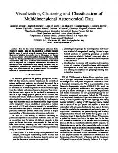
Fig. 2. 3-D plot of music from the three periods of Beethoven. The pieces of music used are listed in table 4.

From each period, we have chosen a number of works from Beethoven as outlined in table 4, and we have calculated an IC distribution for each piece, as described in section 2.1. Each piece can now be visualized as a point in a sixdimensional space, using the values of the IC’s as dimension. For convenience, however, we have chosen three ICs to serve as dimensions. In figure 2, we have visualized the chosen pieces as points in a 3D space. We see that the pieces from the three different periods differ most on the dimension of IC6. Pieces from the early period contain a relatively high percentage of IC6, pieces from the middle period a moderate percentage of IC6, and pieces from the late period a relative low percentage of IC6. In more musical terms, this means that Beethoven has been using relatively many intervals of tritones in his early works, and relatively few tritones in his late works. Of course, these differences in the use of tritones do not characterize entirely the differences between the three periods of Beethoven. However, the fact that a visual classification on the basis of this category is possible, suggests that the use of tritones contributes to the well-known classification of Beethovens music into three periods.

Clustering and classification of music by interval categories

7

Table 4. List of pieces of music by Beethoven used for figure 2. piece of music piano sonata Pathetique part 1 Period 1 piano concerto 2 part 1 symphony 1 part 1 symphony 5 part 1 piano sonata Waldstein part 1 Period 2 string quartet no 11 violin concerto part 1 symphony 6 part 2 symphony 9 part 4 Period 3 piano sonata 29 part 1 piano sonata 31

5

acronym PiSonPathP1 PiConc2P1 Symph1P1 Symph5P1 PiSonWaldP1 StrQuar11 ViolConcP1 Symph6P2 Symph9P4 PiSon29P1 PiSon31

Composer clustering

Western art music, also referred to as classical music, is generally grouped into several musical periods (listed in table 5) and is known to express different characteristics for every period. Using the IC distributions, we have tried to visually cluster several composers and to see if the various musical periods can be visualized in clusters. The composers we have used are listed in table 5. For each composer we have selected around five pieces of music, thereby trying to have some variety in the type of pieces (e.g. symphony, piano sonata, etc.) and the date of composition. The Medieval period we have treated as one item, since for most medieval music the composers are unknown. In the Baroque, Classical and Romantic periods, a distinction can be made between music in a major and music in a minor mode. Since the mode has been shown to influence the IC distribution [6], we have chosen to only choose music in major mode for the present visualisation purpose. Each composer is represented by an IC distribution that was calculated using the selected music. The six interval categories give rise to six dimensions, but we only chose three of these (IC3, IC4 and IC5) to visualize the composers in, see figure 3. Most points (representing the composers) can be found in a region that stretches from a high value for IC5 and low values for IC3 and IC4, to a low value for IC5 and high values for IC3 and IC4. It is interesting to note that the points are not distributed over the entire space but that there is a clear region where they are located. The Baroque period, represented by the composers Bach, Vivaldi and H¨ andel, can be distinguished clearly from the rest of the music. The combined Classical and Romantic period can be distinguished from the rest of the music as well, although it is hard to separate the Classical from the Romantic period. The composers within these periods are quite mixed with each other. The atonal music, a separate area within the modern period, represented by the composers Schoenberg and Webern, are visually distinct from

8

Aline Honingh and Rens Bod Table 5. Periods of European art music and the composers we used for figure 3. musical period Medieval Renaissance Baroque Classical Romantic

Modern

date 500-1400 1400-1600 1600-1750

composers (abbreviation) (various) Palestrina (Pal) Bach (Ba), H¨ andel (Ha), Vivaldi (Vi) 1750-1830 Haydn (Hay), Mozart (Mo), Beethoven (Be), Schubert (Schu) 1830-1900 Brahms (Bra), Mahler (Ma), Tchaikovsky (Tchai), Debussy (De), Mendelssohn (Men), Sibelius (Sib) 1900–. . . Ravel (Ra), Stravinsky (Stra), Schoenberg (Schoe), Webern (Web)

the other composers, which is in accordance with fact that atonal music is musically different from tonal music. Palestrina’s and Medieval music are, according to figure 3, distinct from each other, as well as from both Baroque music and Classical/Romantic music, although the distance to Baroque music is smaller. These observations are consonant with the position of Palestrina’s and Medieval music on the time line of musical periods. Stravinsky can be found halfway between the Classical/Romantic period and the atonal music, which characterizes Stravinsky’s music quite well, having used polytonality and serial techniques in some of his works.

6

Genre classification

We have seen that our method can visualize classical music in a 3D space, roughly separating between the different musical periods. Now we wonder if our method can also distinguish between two broad musical genres: Jazz and Rock. Jazz is a musical tradition and style that employs characteristics like blue notes, improvisation, polyrhythms, syncopation, and the swung note [18]. Rock music is a genre of popular music of which the sound often evolves around guitars, drums, and keyboard instruments and typically uses few chords, simple unsyncopated rhythms, and a backbeat [21]. The pieces of Rock and Jazz music we have used for this experiment are listed in table 6. Each piece of music corresponds to percentages for the six IC’s. As in the previous section, we have chosen IC3, IC4 and IC5 to represent the three dimensions we visualize the different pieces of music in, see figure 4. Looking at figure 4, we can identify two broad regions representing Jazz and Rock music respectively. The clustering is reasonable but not perfect: two songs from the Rock genre are mixed with some of the Jazz songs. Still, it is interesting to find that such a broad classification can be made only on the basis of intervals,

Clustering and classification of music by interval categories

9

90 Bama

80

Hama Pal

Vima

70

Dema Moma Mama Hayma Sibma Bema Men Schuma ma Brama a Tchai Ra m

IC5

60 Medieval

50 40

ma

30 Stra 20

Schoe Web

10 0 0

10

20

20

10

0

30

30

IC4 IC3

(a)

Bama

Vima

100

Hama

80

Medieval Dema

IC5

60

Pal

Mama Mo

ma

Hayma Bema Schuma

Sibma

40 MenRa ma ma

20 Stra 0 0

Bra Tchai a mam

Schoe 0

Web

10

10 20

20 30

30

IC4

IC3

(b)

Fig. 3. 3-D plot of music from composers listed in table 5, viewed from two different angles. The label ‘ma’ indicates the major mode.

especially given the fact that the two genres may be more easily distinguished in the rhythm domain.

10

Aline Honingh and Rens Bod

Rock Jazz

100 90

BeatlElea HendrixJoe

80

ClaptonCoca DireStMoney

IC5

70 60 DavisMileSt

50

HenkdrixVoo MetalOne

40 30

GershSummer ColtrBird ParkerYard DavisSolar BeatlMich ColtrImpres ClaptonLayla

ColtrBlue

20 10 35

40

DavisSoWhat 30

25

20

15

10 IC4

20 5

0

0 IC3

Fig. 4. 3-D plot of Jazz and Rock music, listed in table 6.

7

Conclusions

We have presented a new approach to algorithmic clustering in music based on interval categories (IC’s). With this approach we have been able to successfully distinguish tonal from atonal music in a classification task. In a different application, the three different periods in Beethovens compositions have been visually modeled, and it turned out that the periods could be distinguished from each other along the dimension of IC6. Since this dimension is related to the intervals of tritones we can conclude that the three periods of Beethoven can be characterized (among others) on the basis of the number of tritones. In a third application we have visualized a large number of composers from Western art music on the basis of three dimensions of the IC distribution of their music. In the visualisation we located clear areas for Baroque music and atonal music. Classical and Romantic music could be found in a combined area. In the last application we have visualized a number of Jazz and Rock songs, applying the same method. A reasonable clustering resulted, indicating two broad regions corresponding to Jazz and Rock music. We have shown that musical clustering on the basis of interval categories is possible on many levels, ranging from a general level, where distinctions between broad genres can be made (tonal-atonal/jazz-rock) to a more specific level where distinctions between different pieces from one composer can be made (Beethovens three periods). We should not forget that these IC clusterings are only based on pitch intervals and therefore can never capture all of the differences and commonalities of the investigated music. However, it is striking that a classification can be made with the use of this simple method and thus the approach provides a simple and

Clustering and classification of music by interval categories

11

Table 6. List of Rock and Jazz pieces used for figure 4. piece of music Beatles: Eleanor Rigby Beatles: Michelle Dire Straits: Money for nothing Rock Eric Clapton: Cocaine Eric Clapton: Layla Jimi Hendrix: Hey Joe Jimi Hendrix Voodoo Chile Metallica: One John Coltrane: Blue train John Coltrane: Impressions John Coltrane: Lazy Bird Jazz Miles Davis: Milestones Miles Davis: So What Miles Davis: Solar Charlie Parker: YardBird suite Gershwin: Summertime

acronym BeatlElea BeatlMich DireStMoney ClaptonCoca ClaptonLayla HendrixJoe HendrixVoo MetalOne ColtrBlue ColtrImpres ColtrBird DavisMileSt DavisSoWhat DavisSolar ParkerYard GershSummer

powerful representation of music that can be used to investigate musical similarity on the basis of tonalness, genre, composer, musical period and possibly more.

References 1. Chai, W., Vercoe, B.: Folk music classification using hidden markov models. In: Proceedings of International Conference on Artificial Intelligence (2001) 2. Cilibrasi, R., Vitanyi, P., de Wolf, R.: Algorithmic clustering of music based on string compression. Computer Music Journal 28(4), 49–67 (2004) 3. Forte, A.: The Structure of Atonal Music. New Haven: Yale University Press (1973) 4. Hanson, H.: Harmonic Materials of Modern Music. New York: Appleton-CenturyCrofts (1960) 5. Hillewaere, R., Manderick, B., Conklin, D.: String quartet classification with monophonic models. In: ISMIR 2010:11th International Society for Music Information Retrieval Conference. Utrecht, Netherlands (2010) 6. Honingh, A.K., Bod, R.: Pitch class set categories as analysis tools for degrees of tonality. In: Proceedings of ISMIR. Utrecht, the Netherlands (August 9-13 2010) 7. Honingh, A.K., Weyde, T., Conklin, D.: Sequential association rules in atonal music. In: Proceedings of Mathematics and Computation in Music (MCM2009). New Haven, USA, June 19-22 (2009) 8. Isaacson, E.J.: Similarity of interval-class content between pitch-class sets: the IcVSIM relation. Journal of Music Theory 34, 1–28 (1990) 9. Izmirli, O.: Tonal-atonal classification of music audio using diffusion maps. In: Proceedings of ISMIR 2009. pp. 687–691 (2009)

12

Aline Honingh and Rens Bod

10. Kerman, J., Tyson, A., Burnham, S.G., Johnson, D., Drabkin, W.: Beethoven, Ludwig van. In: Grove Music Online. Oxford Music Online. http://www. oxfordmusiconline.com/subscriber/article/grove/music/40026pg11 (2011), accessed January 11, 2011 11. Morris, R.: A similarity index for pitch-class sets. Perspectives of New Music 18, 445–460 (1980) 12. Perez-Sancho, C., Rizo, D., Inesta, J.: Genre classification using chords and stochastic language models. Connection Science 21(2-3), 145–159 (2009) 13. Quinn, I.: Listening to similarity relations. Perspectives of New Music 39, 108–158 (2001) 14. Rahn, J.: Relating sets. Perspectives of New Music 18, 483–498 (1980) 15. Rogers, D.W.: A geometric approach to pcset similarity. Perspectives of New Music 37(1), 77–90 (1999) 16. Schuijer, M.: Atonal music: Pitch-Class Set Theory and Its Contexts. University of Rochester Press (2008) 17. Scott, D., Isaacson, E.J.: The interval angle: A similarity measure for pitch-class sets. Perspectives of New Music 36(2), 107–142 (1998) 18. Shipton, A.: A New History of Jazz. Continuum, 2nd edn. (2007), pp. 4-5 19. Temperley, D.: The tonal properties of pitch-class sets: Tonal implication, tonal ambiguity and tonalness. Tonal Theory for the Digital Age (Computing in Musicology) (15), 24–38 (2007) 20. Weyde, T.: Modelling cognitive and analytic musical structures in the MUSITECH framework. In: UCM 2005 5th Conference ”Understanding and Creating Music”, Caserta, November 2005. pp. 27–30 (2005) 21. Wilton, P.: Rock. In: the Oxford Companion to Music, Oxford Music Online. http://www.oxfordmusiconline.com/subscriber/article/opr/t114/e5702 (2011), accessed January 31, 2011