Diabetes, Glass, Heart, Heartc, and Horse. The characteristics of the classification problems are summarized in Table 1, which shows considerable diversity in ...
WCCI 2012 IEEE World Congress on Computational Intelligence June, 10-15, 2012 - Brisbane, Australia
IJCNN
Clustering and Selection of Neural Networks Using Adaptive Differential Evolution Tiago P. F. de Lima, Adenilton J. da Silva, and Teresa B. Ludermir Center of Informatics, Federal University of Pernambuco Av. Jornalista Anibal Fernandes, s/n CEP 50.740-560, Cidade Universitária, Recife - PE, Brazil {tpfl2,tbl,ajs3}@cin.ufpe.br strategy has been achieving growing support because of its successful performance, mainly when applied in complex problems [1],[3],[4]. DCS attempts to predict which single classifier is most likely to be correct for a given sample. Only the output of the selected classifier is considered in the final decision, aiming for a new potential mechanism compared to CF [5] which explores the properties of the oracle concept.
Abstract — This paper explores the automatic construction of multiple classifiers systems using the selection method. The automatic method proposed is composed by two phases: one for designing the individual classifiers and one for clustering patterns of training set and search specialized classifiers for each cluster found. The performed experiments adopted the artificial neural networks in the classification phase and k-means in clustering phase. Adaptive differential evolution has been used in this work in order to optimize the parameters and performance of the different techniques used in classification and clustering phases. The experimental results have shown that the proposed method has better performance than manual methods and significantly outperforms most of the methods commonly used to combine multiple classifiers using the fusion version for a set of ૠ benchmark problems.
The CMC involves difficulties related to the amount and types of classifiers, the correct adjustment of classifiers parameters, size of dataset, presence of noise, and other [1]. Even with these difficulties, good results were found with the CMC compared to a single classifier. The hybridization with Evolutionary Algorithm (EA) was proposed to improve the performance of CMC. This proved effective in improving performance in comparison with manual methods of trial and error [6]. Hybridization of the CMC and EA is influenced by the following points: (i) there are many parameters to be defined; (ii) the search by trial and error is difficult and not very productive; and (iii) the good performance achieved by EA in the search involving multiple objectives or parameters [3],[7].
Keywords: Combinations of Multiple Classifiers, Classifier Selection, Clustering and Selection, Artificial Neural Networks, K-means, Adaptive Differential Evolution.
I.
INTRODUCTION
Let ܦൌ ሼܦଵ ǡ ܦଶ ǡ ǥ ǡ ܦ ሽ be a set of ܮclassifiers and ȳ ൌ ሼ߱ଵ ǡ ߱ଶ ǡ ǥ ǡ ߱ ሽ be a set of ܥlabels. Each classifier gets as its input a feature vector ࢞ אԸ and assigns it to a class label from�ȳ, i.e., ܦ� ǣ�Ը ՜ ȳ. In many cases the classifier output is a ܥ-dimensional vector with supports to the ܥclasses, for instance, ்
ܦ ሺ࢞ሻ ൌ ൣ݀ǡଵ ሺ࢞ሻǡ ݀ǡଶ ሺ࢞ሻǡ ǥ ǡ ݀ǡ ሺ࢞ሻ൧ ��������������������������������
Despite improvements in the final performance, the hybridization of CMC with EA causes an increasing in the number of difficulties related to define the parameters of EA such as: (i) choice of algorithms (Artificial Immune System, Differential Evolution, Evolution Strategies, Genetic Algorithm, Particle Swarm Optimization, etc); (ii) generic choice of algorithm parameters (population size, stopping criterion, fitness function, codifications, etc); and (iii) specific parameters to the chosen EA (crossing rate, selection pressure, etc) [8]. Despite these limitations, the application of EA on CMC has produced good results. This is encouraging for this line of research [1],[4].
(1)
Without loss of generality, we can restrict ݀ǡ ሺ࢞ሻ within the interval �ሾͲǤͲǡͳǤͲሿ , ݅ ൌ ͳǡ ʹǡ ǥ ǡ �ܮand �݆ ൌ ͳǡ ʹǡ ǥ ǡ ܥ. Thus, ݀ǡ ሺ࢞ሻ is the degree of support given by classifier ܦ to the hypothesis that ࢞ comes from class�߱ . Combining classifiers means to find a class label for ࢞ based on the ܮclassifier outputs �ܦଵ ሺ࢞ሻǡ ܦଶ ሺ࢞ሻǡ ǥ�ܦ ሺ࢞ሻ . In doing so, we weigh the individual opinions through some thought process to reach a final decision that is presumably the most informed one [1]. This strategy refers to human nature and tends to produce positive results mainly when there is a set of reliable classifiers with diverse knowledge, followed by a fair and efficient combination scheme.
Most of the discussions and design methodologies of CMC are devoted to fusion version and are concerned with how to achieve good performance by creating diversity measure and combination schema. Research is less common in Clustering and Selection (CS) methodology. Basically, the methodology of CS is first to cluster the training set and subsequently find a specialized classifier for each cluster. Such methodology was first implemented by Kuncheva [9], who worked with a predefined number of clusters and classifiers parameters. The focus of this paper is to propose an automatic method (CSJADE) to CMC using the selection method through CS methodology with Adaptive Differential Evolution (JADE). The preference for JADE was motivated by the simulations
There are generally two types of Combinations of Multiple Classifiers (CMC): Classifier Fusion (CF) and Dynamic Classifier Selection (DCS) as named in [2]. In CF, individual classifiers are applied in parallel and their outputs are combined in some way to achieve a "group consensus". This
U.S. Government work not protected by U.S. copyright
747
כ כ ܲ σ ୀଵ ܲሺܴ ሻ ܲ൫ ܦหܴ ൯ ൌ ܲሺ ܦሻ
results that showed the JADE is better than, or at least comparable to, other classic or adaptive differential evolution algorithms, the canonical particle swarm optimization, and other EA from the literature [10],[11]. For the classification phase the preference for Artificial Neural Networks (ANN) was motivated by the success in many types of problems with degrees of complexity and different application fields [12],[13]. In the clustering phase, the k-means algorithm was chosen because it is the most popular clustering techniques in addition to being fast and easy to implement [14]. II.
(4)
Equation (4) shows that the combined scheme performs equal or better than the best classifier כ ܦin the pool ܦ, regardless of the way the features space has been partitioned. The only condition is to ensure that ܦሺሻ is the best among the ܮclassifiers in ܦfor region ܴ . III.
ADAPTIVE DIFFERENTIAL EVOLUTION
According to [15], DE is a population of candidate solutions, chosen randomly in the search space, represented by�ࡼீ ൌ ሼࢄǡீ ǡ ݅ ൌ ͳǡʹǡ ǥ ǡ ܰܲሽ, where ܩis the index of the current generation, ݅ is the index of the individual and ܰܲ is the population size. Each individual is a ܦ-dimensional vector represented as follows: �ࢄǡீ ൌ ሼݔǡǡ ǡ ݆ ൌ ͳǡʹǡ ǥ ǡ ܦሽ , where ݔǡǡ is the attribute ݆ of individual ݅ in generation ܩ. In each generation, mutation, crossover and selection operators affect the population until achieving the stopping criterion, as show in Algorithm 1.
A PROBABILISTIC VIEW
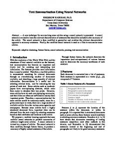
The construction of a DCS can be accomplished by grouping the training set regardless of the labels of the classes in ܭ ͳ regions denoted by �ܴଵ ǡ ܴଶ ǡ ǥ ǡ ܴ . An example of partitioning into regions is show in Figure 1.
Algorithm 1 - Differential Evolution 1: 2: 3: 4: 5: 6: 7: 8: 9: 10: 11: 12: 13: 14: 15: 16: 17: 18: 19: 20: 21: 22: 23: 24: 25: 26: 27: 28: 29: 30: 31: 32:
Figure 1 – An example of partitioning the features space in ব with two classification regions into three selection regions.
During training of the DCS we decide which classifier from ܦwe should designate for each region in�ܴ. Thus, the number of classifiers ܮis not necessarily equal to the number of regions�ܭ. Also, some classifiers might never be designated and therefore they are not needed in the DCS. Even the classifier with the highest average accuracy over the whole features space might be dropped from the final set of classifiers. On the other hand, one classifier might be designated for more than one region. Let �ܦ א כ ܦbe the classifier with the highest average accuracy over the whole features space �Ը . Denote by ܲ൫ܦ หܴ ൯ the probability of correct classification by ܦ in region ܴ Ǥ Consider ܦሺሻ ܦ אthe classifier responsible for region�ܴ �,�݆ ൌ ͳǡ ʹǡ ǥ ǡ ܭ. The overall probability of correct classification of our classifier selection system is
Begin // Inicialization Create a random initial population of ܰܲ individuals // Evaluation Evaluate each individual while termination criterion not met do for ݅� ൌ �ͳ�to ܰܲ // Mutation Select basis vector ࢄ௦௦ǡீ Randomly choose ࢄଵǡீ ് ࢄ௦௦ǡீ Randomly choose ࢄଶǡீ ് ࢄଵǡீ ് ࢄ௦௦ǡீ Calculate the vector donor ࢂǡீ ൌ ࢄ௦௦ǡீ ܨሺࢄଵǡீ െ ࢄଶǡீ ሻ // Crossover ݆ௗ ൌ ݐ݊݅݀݊ܽݎሺͳǡ ܦሻ for ݆� ൌ �ͳ�to ܦ if ݆� ൌ �݆ ݀݊ܽݎor ݀݊ܽݎሺͲǡͳሻ ݎܥ ݑǡǡ ൌ �� ݒǡǡ else ݑǡǡ ൌ �� ݔǡǡ end end // Evaluation Evaluate the new individual ࢁǡீ // Selection if ݂ሺࢁǡீ ሻ� ݂ሺࢄǡீ ሻ ࢄǡீାଵ ൌ � ࢁǡீ else ࢄǡீାଵ ൌ � ࢄǡீ end end end end
The JADE algorithm was proposed in 2009 by Zhang and Sanderson [11] with a new mutation strategy called �ܧܦȀ ܿ ݐ݊݁ݎݎݑെ ݐെ ݐݏܾ݁, which uses an optional file, and an adaptation of the parameters ( ܨdifferential weight) and ݎܥ (crossover probability). The mutation strategy JADE is described in equation (5), where is in the interval�ሾͲǤͲǡ ͳǤͲሿ, ࢄ௦௧ǡீ is chosen from the ͳͲͲΨ best individuals in the current generation, ܨ is associated with ࢄǡீ and it is
ܲ ൌ σ ୀଵ ܲ൫ܴ ൯ܲ ൫ܴ ൯ ൌ σୀଵ ܲ൫ܴ ൯ܲሺܦሺሻ ȁܴ ሻ������������������(2)
where ܲ൫ܴ ൯�is the probability that an input ࢞ drawn from the distribution of the problem falls in ܴ . To maximize�ܲ , we assign ܦሺሻ so that ܲ൫ܦሺሻ หܴ ൯ ܲ൫ܦ௧ หܴ ൯ǡ ݐ�ൌ ͳǡ ǥ ǡ ( ����������������������������������ܮ3) Thus, from equations (2) and (3), we have that
748
determined at each generation, ࢄଵǡீ is randomly selected from the current population and ࢄଶǡீ is randomly selected from the population (JADE without file) or from the union of the population and one file (JADE with file). In the beginning of the algorithm the file is empty and when a parent solution ࢄǡீ loses your position, it is added to the file. When the size of file is bigger than�ܰܲ, one solution is randomly removed from the file. The advantage in use the file is to keep the diversity, increasing the amount of available information.
ࢂǡீ ൌ ࢄǡீ ܨ ൫ࢄ௦௧ǡீ െ ࢄǡீ ൯ ܨ ൫ࢄଵǡீ െ ࢄଶǡீ ൯
second component and so on. If two or more attributes have the same value, it will be considered the attribute with the smallest index. The selected training algorithm is executed up to ͷ epoch. The second part involves the parameter values from the training algorithm specified in the previous part. Each parameter has a predetermined position, therefore when the algorithm is chosen, it is possible recover: (i) learning rate and momentum, for the BP; (ii) learning rate, increment to weight change, decrement to weight change, initial weight change and maximum weight, for the RPROP; (iii) initial ݉ݑ, ݉ ݑdecrease factor, ݉ ݑincrease factor and maximum ݉ݑ, for the LM; and (iv) change in weight for second derivative approximation (ߪ) and regulating the indefiniteness of the Hessian (Ȝ), for the SGC. All parameters of this part have real values, but they are not directly encoded. They are initialized between ሾെͳǤͲǡ ͳǤͲሿ and a linear map is used to obtain the real values of the parameters.
(5)
The parameters ݎܥand ܨare calculated for each individual in the population. The value of ݎܥ is calculated using equation (6) and then truncated to ሾͲǤͲǡͳǤͲሿ, where ݊݀݊ܽݎሺɊݎܥǡ ͲǤͳሻ is a random number following normal distribution with mean Ɋݎܥ and standard deviation ͲǤͳ. The value of ܨ is calculated using equation (7), where ܿ݀݊ܽݎሺɊܨǡ ͲǤͳሻ is a random number following Cauchy distribution with mean Ɋ ܨand standard deviation�ͲǤͳ. If the generated value is bigger than�ͳ, it will assume the value �ͳ , and if it is lower than �Ͳ , it will be regenerated. ݎܥ ൌ ݊݀݊ܽݎሺɊݎܥǡ ͲǤͳሻ
(6)
ܨ ൌ ܿ݀݊ܽݎሺɊܨǡ ͲǤͳሻ
(7)
The third part is responsible for the process of selecting a subset of features extracted from the original set, in order to reduce the dimensionality of the problem and consequently the complexity of ANN generated. Therefore, the number of attributes of this part depends on the problem and each feature is defined in the input layer if its attribute is a positive value. Although the number of neurons in the output layer has not changed during the process, it is also dependent of the problem and is defined by the winner-takes-all, in which the output neuron with the highest value determines the class pattern. Thus, the number of neurons in the output layer of the ANN is equal to the number of classes of the problem.
The values of Ɋ ݎܥand Ɋ ܨare updated in each generation as described in equations (8) and (9), where ݉݁ܽ݊ ሺǤ ሻ is the usual arithmetic mean and ݉݁ܽ݊ ሺǤ ሻ is the Lehmer mean. The values of �ܵ and ܵி are respectively the set of all successful mutation factors at the last generation. Ɋ ݎܥൌ ሺͳ െ ܿሻǤ Ɋ ݎܥ ܿǤ ݉݁ܽ݊ ሺܵ ሻ
(8)
Ɋ ܨൌ ሺͳ െ ܿሻǤ Ɋ ܨ ܿǤ ݉݁ܽ݊ ሺܵி ሻ
(9)
IV.
The fourth part has dimension equal to the maximum number of hidden layers, in this work equal to ͵. According to [23], from extension of the Kolmogorov theorem, we need at most two hidden layers, with a sufficient number of units per layer to produce any mappings. It was also proved by [23] that only one hidden layer is sufficient to approximate any continuous function. Nevertheless, in complex problems the use of three hidden layers can facilitate and improve the generalization of ANN. To determinate the number of hidden layers of the ANN is considered the attribute with the most representative value. If this value is the first attribute then the ANN has only one hidden layer, if it is the second attribute then the ANN has two layers, and so on.
ARTIFICIAL NEURAL NETWORKS OPTIMIZATION
The performance of an ANN is affected by several factors, including the training algorithm, the parameters of the training algorithm, the features selection, the number of hidden layers and neurons for layer, the transfer functions and the initial weights. This means its proper definition is considered an NPHard problem [16]. Thus, for the construction phase of the components of the set�ܦ, the JADE algorithm was used for ͳͲͲ generations with ͵ͷ individuals randomly generated through a direct encoding scheme, inspired in the works of [17] and [18], as show in Figure 2. training algorithm
training algorithm parameters
inputs
layers
neurons
transfer functions
The fifth part encodes the number of hidden neurons in each layer. This part considers the maximum number of neurons per layer equal to �݊ , where the first ݊ attributes correspond to the first layer and the number of neurons is defined by the position of the attribute value that is more representative. The next ݊ attributes correspond to the second layer, and so on. Thus the number of attributes of this part is fixed and equal to the maximum number of layers multiplied by the maximum number of neurons per layer. The literature states that the best networks are those with a small number of neurons [24], so we use the maximum number of neurons per layer equal to ͳͲ.
initial weights
Figure 2 – Composition of an individual in ANN optimization
In the first part of these individuals, there is information on the training algorithm type. Such information is stored using the continuous values in which the most representative value indicates what training algorithm will be used to train the ANN, such as: Backpropagation (BP) [19], Resilient Backpropagation (RPROP) [20], Levenberg-Marquardt (LM) [21] and Scaled Conjugate Gradient (SGC) [22]. The use of BP is indicated when the highest values are in the first component of this part; RPROP is used when the highest values are in the
The sixth part selects for each hidden layer, through the position of the most representative attribute, one of the following functions: Pure-linear (ܲ ), Tang-sigmoid (ܶ ) and
749
clusters and in this work is equal to ͵Ͳ. A cluster is active if its corresponding attribute is a positive value. The values of the attributes of this part are initialized within the range�ሾെͲǤͷǡ ͲǤͷሿ.
Log-sigmoid ( ) ܮ. To determinate the transfer function is considered the attribute with the most representative value. If this value is the first attribute then the function ܲ is used, if it is the second attribute then the function ܶ is used, and if this value is the third attribute then the function ܮis used. The transfer function of the output layer is always�ܲ.
The second part, with dimension ܭ௫ ൈ ݀ǡ defines the centers of each cluster. Each centroid has a predetermined position, therefore after defining the active clusters, its respective centers can be recovered. The values of the centers are initialized within the range ሾെͲǤͷǡ ͲǤͷሿ and are directly used in the k-means algorithm, which is executed up to ͳͲ epoch.
The last part has fixed dimension, which is calculated according to the number of bias, the maximum number of layers, the maximum number of neurons per layer, the maximum amount of features and class labels. The weights are directly encoded on the individuals and they are initialized in the range�ሾെͳǤͲǡ ͳǤͲሿ . Baldwin's method was used, i.e., the weights changed by the training algorithm do not return to the individual.
The last part considers the size ܮof the set ܦbuilt up in the previous step. The first ܮattributes correspond to the designated for the first region that is defined by the position of the more representative attribute value. The next ܮattributes correspond to the second region, and so on. Therefore, this part has dimension�ܭ௫ ൈ ܮ.
The evaluation function shown in equation (10) is composed of five pieces of information: ܫ௩ - validation error; ܫ௧ - training error; ܫௗ - number of hidden layers; ܫௗ – total number of hidden neurons; and ܫ௨ - weight of transfer functions (ܲ with ͲǤʹ, ܶ with ͲǤ͵ e ܮwith ͲǤͷ).
The evaluation function shown in equation (11) is composed of two pieces of information: ܫ௧ - mean classification error of the training set and ܫ௩ - mean classification error of the validation set.
ܫ௧ ൌ ߙ ܫ כ௩ ߚ ܫ כ௧ ߛ ܫ כௗ ߜ ܫ כௗ ߝ ܫ כ௨ (10)
ܫ௧ ൌ ߙ ݏܾܽ כሺܫ௧ െ ܫ௩ ሻ ߚ ܫ כ௧ ���
In equation (10), the constants�ߙ,�ߚ,�ߛ,�ߜ and ߝ have values between ሾͲǤͲǡͳǤͲሿ and control the respective factors upon the overall fitness calculation process. The constants were found empirically by [18] as follows: �ߙ ൌ ͲǤͺ , �ߚ ൌ ͲǤͳͶͷ , �ߛ ൌ ͲǤͲ͵,�ߜ ൌ ͲǤͲͲͷ and ߝ ൌ ͲǤͲʹ. These definitions imply that when apparently similar individuals are found, those that have the least training error, structural complexity, and transfer function complexity will prevail. The ܫ௩ and ܫ௧ values are calculated using equation (11), where ܰ and ܲ are the total number of outputs and number of training patterns, respectively; ݀ and are the desired output (target) and network output (obtained), respectively. ܫ௦ ൌ
ଵ ே
V.
ଶ σୀଵ σே ୀଵሺ݀ െ ሻ
In equation (11), the constants ߙ and ߚ control the influence of the respective factors upon the overall fitness calculation process and were empirically defined as follows: ߙ ൌ ͲǤ͵ and ߚ ൌ ͲǤ. The ܾܽݏሺǤ ሻ�is the absolute value. VI.
(11)
Table 1 – Characteristics of data sets used in the experiments.
The project for the development of a DCS basically takes into account the definition of the strategy of selection classifiers which will compose the system. Therefore, there is need to create a mapping of the input signals on the type of signal that a given classifier can respond with an acceptable quality. This mapping can be viewed as a task of partitioning the information into regions or clusters. Thus, for each region, where data are organized by neighborhood, a classifier is designated. In this way, for selecting a classifier responsible for each region, using the CS methodology, the JADE algorithm was employed for ͳͲͲ generations with ͷͲ individuals randomly generated following a coding scheme inspired by [25], as show in Figure 3. cluster centroids
EXPERIMENTS AND RESULTS
To ensure the efficiency of the CSJADE, the experiments were conducted using well-know classification problems found in the UCI repository [26]. They are: Cancer, Card, Diabetes, Glass, Heart, Heartc, and Horse. The characteristics of the classification problems are summarized in Table 1, which shows considerable diversity in the number of examples, features and classes among problems.
CLUSTERING AND SELECTION OPTIMIZATION
activation threshold
(11)
No. of Problem examples
features
classes
Cancer
699
9
2
Card
690
51
2
Diabetes
768
8
2
Glass
214
9
6
Heart
920
35
2
Heartc
303
35
2
Horse
364
58
3
designated
Figure 3 – Composition of an individual in CS optimization
The first part of these individuals controls, through the first ܭ௫ attributes of the individual, which are the active clusters in k-means algorithm. ܭ௫ is the maximum number of
750
A total of ͳͲ iterations using different divisions were used for each base. The data were randomly divided by the stratification into ͲΨ for training and ͵ͲΨ for testing. The first part was the input for the Algorithm 2 (ͲΨ for training and ͵ͲΨ for the validation set) and the other part was used only to test the final solution.
Table 2 – Mean classification error considering interactions. CMC CSJADE
ADBO
BAG
MB
MLP
Cancer
0.0301 (0.0116)
0.0368 (0.0144)
0.0368 (0.0115)
0.0335 (0.0101)
0.0421 (0.0147)
Card
0.1232 (0.0279)
0.1657 (0.0283)
0.1367 (0.0167)
0.1633 (0.0248)
0.1662 (0.0285)
Diabetes
0.2265 (0.0196)
0.2652 (0.0374)
0.2569 (0.0286)
0.2404 (0.0277)
0.2609 (0.0418)
Glass
0.3400 (0.0540)
0.3230 (0.0580)
0.3308 (0.0785)
0.3369 (0.0865)
0.3431 (0.0891)
Heart
0.1721 (0.0221)
0.2181 (0.0114)
0.1804 (0.0145)
0.1956 (0.0153)
0.2199 (0.0127)
Heartc
0.1736 (0.0343)
0.2242 (0.0312)
0.1967 (0.0317)
0.2307 (0.0439)
0.2209 (0.0409)
Horse
0.3376 (0.0302)
0.3670 (0.0394)
0.3449 (0.0341)
0.3541 (0.0382)
0.3660 (0.0322)
Mean
0.2004
0.2286
0.2119
0.2221
0.2313
Algorithm 2 – Construction of the model CSJADE 1: 2:
3:
Develop the individual classifiers ܦଵ ǡ ܦଶ ǡ ǥ ǡ ܦ by JADE using the labeled training set. Disregard the class labels, use JADE to optimize the clustering of training set into ݇ regions by k-means and designate the classifier ܦሺሻ for each region ܴ . Return the centroids ݒଵ ǡ ݒଶ ǡ ǥ ǡ ݒ and the classifiers with better accuracy for each region ܦሺଵሻ ǡ ܦሺଶሻ ǡ ǥ ǡ ܦሺሻ
The set of classifiers ܦin Algorithm 2 was formed by all individuals of the last generation in the ANN optimization phase. To achieve diversity and experts in certain areas, manipulations in training set with the supply of random samples with replacement were used for the construction of each classifier�ܦ ܦ א. This causes individual training subsets to overlap significantly, with many of the same instances appearing in most subsets, and some instances appearing multiple times in a given subset. One important point using this strategy, called bagging, is the fact that the ANN are unstable classifiers. A classifier is considered unstable if small perturbations in the training set results in large changes in the constructed predictor [27]. Algorithm 3 shows how the selection is made during operation of the model CSJADE to predict which single ANN is most likely to be correct for a given sample.
These results suggest that performance of CSJADE is significantly better than a single classifier (SC). Moreover, its mean accuracy was also better or equivalent when compared to classical techniques for the CMC. This shows the potential of CS method when EA are correctly employed to optimize clustering and classification techniques. The main disadvantage of the CSJADE method, as show in Table 3, is that performing the search is very time consuming in comparison with the classical methods. The time is related to the search performed in one interaction of the each problem, measured in minutes of processing on a computer with Microsoft Windows operational system, ͺǤͲ GB of RAM and a processor Intel Xeon of ͵ǤͲ GHz.
Algorithm 3 – Operation of the model CSJADE 1: 2:
SC
Problem
Given the input�࢞ אԸ , find the nearest cluster center from�ݒଵ ǡ ݒଶ ǡ ǥ ǡ ݒ , say, ݒ . Use ܦሺሻ to label�࢞.
Table 3 – Mean time of processing for one interaction. Time in minutes Problem
Table 2 presents the performance obtained with the means of the classification errors of ͳͲ runs with the test set during the operation of CSJADE, executed in Matlab 2009, and some classical methods for the construction of classifier systems. The classical methods considered in these experiments, executed in Java language with Weka 3.6.6, were bagging (BAG) [28], MultiBoosting [29] (MB), AdaBoost.M1 [30] (ADBO) and single Multilayer Perceptron [31] (MLP). The results were expressed as follows: ݉݁ܽ݊�ሺ݊݅ݐܽ݅ݒ݁݀�݀ݎܽ݀݊ܽݐݏሻǤ To determine whether the differences among the methods were statistically significant, we used the Bootstrap Hypothesis Test with ͳͲΨ of significance. The boldface result means that the method is better than the others with same output type. The emphasized results mean that there is no difference between the emphasized method and boldfaced method.
751
CSJADE
ADBO
BAG
MB
MLP
Cancer
23.79 (2.59E+00)
0.0428 (7.99E-03)
0.0438 (1.58E-04)
0.0437 (1.98E-04)
0.0044 (4.60E-05)
Card
28.21 (3.61E+00)
0.2477 (9.04E-02)
0.5502 (3.02E-03)
0.2908 (1.46E-01)
0.0548 (3.32E-04)
Diabetes
33.21 (2.92E+00)
0.0384 (7.24E-03)
0.0440 (1.36E-04)
0.0438 (1.60E-04)
0.0044 (7.40E-05)
Glass
32.69 (3.62E+00)
0.0206 (3.68E-03)
0.0263 (1.58E-04)
0.0261 (1.66E-04)
0.0026 (8.05E-05)
Heart
28.08 (2.23E+00)
0.2945 (1.07E-01)
0.3912 (1.01E-03)
0.3751 (4.95E-02)
0.0392 (2.17E-04)
Heartc
30.48 (4,06E+00)
0.0651 (5.03E-02)
0.1312 (2.89E-04)
0.0762 (5.86E-02)
0.0132 (6.08E-05)
Horse
37.48 (2.91E+00)
0.2579 (1.25E-01)
0.4228 (2.33E-03)
0.3598 (1.34E-01)
0.0423 (1.91E-04)
Mean
30.56
0.1382
0.2299
0.1736
0.0230
With the evidence of the potential of the proposed DCS method, further implementations may contribute to achieve better results. Some suggestions are: analyze the effect of classifier pool size; test different rules of combination to dynamically select multiple classifiers for each region; check the performance through other means of evolution as the method of Lamarck and also through other EA; investigate techniques for classification and data clustering to get better shape representation of the data distribution and then to improve their classification; review the fitness functions used which may contribute to a significant improvement in performance. In addition to these suggestions, the proposed method can also be extended and applied to regression problems, such as function approximation and prediction of time series.
The length of time required for each execution can be explained by the cost of evaluation function that performs trainings and simulations in each time that it is invoked. Therefore, the execution time increases with the number of attributes and examples of each problem. Thus, for applications with large bases and critical computation time, the proposed method should not be used. However, its performance compared to traditional methods of construction of classifier systems justifies its use in other situations. Table 4 presents the performance of some methods from the literature. The method considered were TD03 [32], TZ03 [33], Dv04b [34], MM04 [35] and CY09 [36]. Comparisons between CSJADE and methods from the literature must be made with caution, because the results are obtained with different experimental model setups as well as with different learning approaches. Thus the highlighted values indicate the method that has the lowest mean classification error for each problem. On average, the CSJADE is situated between the methods with better performances. It is worth mentioning that the purpose of this paper was to explore the potential of CS methodology and not to find the best experimental results.
ACKNOWLEDGMENT The authors would like to thank FACEPE, CNPq and CAPES (Brazilian Research Agencies) for their financial support. VIII. REFERENCES
Table 4 – Comparison with other methods in the literature.
[1] [2]
References Problem CSJADE
TD03
TZ03
Dv04b
MM04
CY09
Cancer
0.0301
-
-
0.0280
0.0318
0.0263
Card
0.1232
0.1433
0.1580
0.1432
0.1261
-
Diabetes
0.2265
0.2372
0.2710
0.2402
0.2448
0.2316
Glass
0.3400
0.3154
0.3800
0.2519
0.2766
-
Heart
0.1721
0.1617
-
0.1605
0.1815
0.1643
[6]
Heartc
0.1736
-
0.2050
0.1620
0.2249
-
[7]
Horse
0.3376
-
0.1910
-
0.2442
-
[3]
[4]
[5]
[8] [9]
VII. CONCLUSION AND FUTURE WORK This paper presents the development of a method that aims to construct automatic DCS applied to supervised classification problems. For this purpose, hybridizations of recent advances in EA with classical algorithms for classification and data clustering have been proposed. The method CSJADE showed to be a promising tool, with good results in comparison with manual search methods and also with other methods commonly used in CMC. However, its main limitation is related to the large amount of time required for the solutions to be found. Even so, good results motivate the continuation of studies to advance the search for more effective methods for the construction of DCS.
[10]
[11]
[12] [13] [14] [15]
752
R. Polikar. "Ensemble based systems in decision makink," IEEE Circuits And Systems Magazine, vol.6, no. 3, pp. 21-45, 2006. K. Woods, W.P.J Kegelmeyer, and K. Bowyer. "Combination of multiple classifiers using local accuracy estimates," IEEE Transactions on Pattern Analysis and Machine Inteligence, vol. 19, no. 4, pp. 405410, 1997. N. García-Pedrajas and C. Fyfe. "Construction of classifier ensembles by means of artificial immune systems," Journal of Heuristics, vol. 14, no. 3, pp. 285-310, 2008. M.D. Muhlbaier, A. Topalis, and R. Polikar. "Learn++.nc: combining ensemble of classifiers with dynamically weighted consult-and-vote for efficient incremental learning of new classes," IEEE Transactions on Neural Networks, vol. 20, no. 1, pp. 152-168, 2009. G. Giancinto and F. Roli. "Methods for dynamic classifier selection", ICPA'99, 10th International Conference on Image Analysis and Processing, Venice, Italy, pp.659-664, 1999. L.I. Kuncheva, Combining Pattern Classifiers, Methods and Algorithms. New York, NY: Wiley-Interscience, 2005. C.A.C. Coelho, D.A.V. Veldhuizen, and G.B. Lamont. Evolutionary algorithms for solving multi-objective problems, vol. 5. Kluwer Academic Publishers, 2002. A.E. Eiben and J.E. Smith. Introduction to evolutionary computing. Springer, 2003. L.I. Kuncheva. Clustering-and-selection model for classifier combination. "Fourth International Conference on Knowledge-Based Inteligent Engineering Systems and Allied Technologies, vol. 1, pp. 185188, 2000. D. Swagatam and N.S. Ponnuthurai. Differential Evolution: A Survey of the State-of-the-Art. IEEE Transactions on Evolutionary Computation, vol. 15, no. 1, pp. 27-54, 2011. J. Zhang and A.C. Saderson. Jade: Adapative differential evolution with optional external archive. Evolutionary Computation, IEEE Transactions on, vol. 13, no. 5, pp. 945-958, 2009. T. Masters. Signal and image processing with neural networks: a C++ sourcebook. John & Sons, Inc., 1994. C.M. Bishop. Neural networks for pattern recognition. Oxford University Press, 1995. A. K. Jain, M. N. Murty, and P. J. Flynn, “Data clustering: A review”, ACM Comput. Surv., vol. 31, no. 3, pp. 264-323, 1999. K.V. Prince, R.M. Storn, and J.A. Lampinen. Differential evolution: a pratical approach to global optimization. Natural Computing Series. Springer-Verlag, Berlin, Germany, 2005.
[16] J.L. Jeffrey and J.S. Vitter. Complexity Results on Learning by Neural Nets, in machine learning, pp. 211-230, 1991. [17] A.J. Silva, N.L. Mineu, and T.B. Ludermir. Evolving artificial neural networks using adaptive differential evolution. Iberamia, vol. 6433, pp.396-405, 2010. [18] L.M. Almeida and T.B. Ludermir. A multi-objective memetic and hybrid metodology for optimizing the parameters and performance of artificial neural networks. Neurocomputing, vol. 73, pp. 1438-1450, 2010. [19] D.E. Rumelhart, G.E. Hinton and R.J. Williams. Learning representations by backpropagation errors. Nature (London), vol. 323, pp. 533-536, 1986. [20] M. Reidmiller and H. Braun. A direct adaptative method for daster backpropagation learning: The rprop algorithm. Proceedings of IEEE Int. Conf. on Neural Networks (ICNN), vol. 16, pp. 586-591, San Francisco, 1993. [21] M. Hagan e M. Menhaj. Training feedforward networks woth the marquardt algorithm. IEEE Transactions on Neural Networks, vol. 5, no. 6, pp. 989-993, 1994. [22] M.F. Mooler. "A scaled conjugate gradient algorithm for fast supervised learning," Neural Networks, vol. 6, pp. 525-533, 1993. [23] G. Cybenko. "Approximation by superpositions of sigmoidal function," Mathematics Control Signals Systems, vol. 2, pp. 303-314, 1989. [24] K.P. Liao e R. Fildes. The accuracy of a procedural approach to specifying feedfoward neural networks for forecasting. Computer & Operations Research, 2005. [25] S. Das, A. Abraham e A. Konar. Automatic clustering using na improved differential evolution algorithm. IEEE Transactions on Systems, Man, and Cybernetics, Part A: Systems and Humans, vol. 38, no. 1, pp. 218-237, 2008. [26] A. Asuncion and D.J. Newman. UCI machine learning repository, 2007. [27] L. Breiman, “Bias, variance, and arcing classifiers,” Tech. Rep., University of California, Berkeley, 1996. [28] L. Breiman, "Bagging predictors," Machine Learning, vol. 26, no. 2 pp. 123-140, 1996. [29] G.I. Webb, "MultiBoosting: A technique for Combining Boosting and Wagging, " Machine Learning, vol. 40, no. 2, pp. 159-196, 2000. [30] Y. Freund and R.E. Schapire. "Experiments with a new boosting algorithm,". Thirteenth International Conference on Machine Learning, Bari, pp. 148-156, 1996. [31] S. Haykin. Neural Networks: a comprehensive foundation. Prentice Hall, 1999. [32] L. Todorovski and S. Dzeroski, "Combining classifiers with meta decision trees," Machine Learning, vol. 50, no.3, pp. 223-249, 2003. [33] K. M. Ting and Z. Zheng. A study of adaboost with naive bayesian classifiers: weakness and improvement. International Journal of Computational Inteligence, vol. 19, no. 2, pp. 186-200, 2003. [34] S. Dzeroski and R. Zenko, "Is combining classifiers with stacking better than selecting the best one?," Machine Learning, vol. 54, no. 3, pp. 255273, 2004. [35] P. Melville and R.J. Mooney, "Creating diversity in ensembles using artificial data," Information Fusion, vol. 6, pp. 99-11, 2004. [36] H. Chen and X. Yao. "Regularized negative correlation learning for neural networks ensembles," IEEE Transactions on Neural Networks, vol. 20, no. 12, pp. 1692-1979, 2009.
753