Feature Selection in Evolved Artificial Neural Networks using the Evolutionary Algorithm EPNet V. Landassuri-Moreno School of Computer Science University of Birmingham Birmingham, B15 2TT UK
[email protected]
Abstract The evolution of Artificial Neural Networks (ANNs) using the EPNet algorithm has given good results in previous publications. However, the input feature selection problem has never been fully considered before, because the inputs were fixed and only the architectures evolved. Thus, in this work is presented an empirical study to determine statistically whether it is better (or not) to evolve the inputs for the EPNet algorithm. To test this, a prediction task was used with 21 Time Series from different dynamics and fields. The results obtained show that the evolution of inputs does improve the performance of the algorithm in some cases, but leads to worse performance in others.
1
Introduction
In previous studies with the EPNet algorithm [11, 12] the user set manually the required number of inputs and then evolved the ANN architectures. In this sense, no input feature selection technique has been used in the EPNet algorithm. Instead, existing domain knowledge was used to chose appropriate inputs before the evolution of the ANNs began, i.e. the input units were fixed throughout the evolution. Elsewhere, feature selection techniques have proved useful because there is always the possibility of presenting redundant or irrelevant inputs to the ANNs, e.g. the information given by them could already be presented in other input units, or they could simply not contribute to solving the problem. Thus, if the information is redundant, it will add nothing to solving the task, and if it is irrelevant, it will not improve the results [3]. Moreover, if input feature selection is not used, it is possible that unnecessary inputs will result in bigger ANNs requiring more time in the training process, or introduce unnec-
John A. Bullinaria School of Computer Science University of Birmingham Birmingham, B15 2TT UK
[email protected]
essary noise into the ANN which will typically result in poorer ANN output performance. Existing feature selection techniques fall into two general categories [3]: Generational procedures and Evaluation function procedures. In both methods, several different variations are used to determine what are the most appropriate inputs to the model. In this work it was decided to not use an Evaluation functions method to determine appropriate inputs, because this procedure adds an extra stage in the solution of the task, i.e. first an appropriate number of inputs has to be determined, and only then is the main procedure applied to solve the problem [5, 8, 9, 14]. This approach has previously been applied to forecasting [5, 8] and to classification [9, 14]. Consequently, the approach adopted in this work belongs to the Generational procedures, because it evolves the ANNs’ inputs with an Evolutionary Algorithm (EA) [2, 7] to allow the automatic adaptation of the inputs at the same time as the rest of the architecture evolves. Since the EPNet algorithm is based on the Evolutionary Programming approach, it only uses mutations to perform the evolution. Therefore, it avoids the well-known evolutionary ANN permutation problem that can arise with crossover operators [11]. Thus, by applying a feature selection technique over the EPNet algorithm, one can have better confidence in the results than if it is applied over an algorithm that is not so good for this task, such as a Genetic Algorithm (GA). In the literature it is possible to find several approaches and combinations of them to solve diverse kinds of problems using feature selection, e.g. leaving the architectures fixed and finding appropriate inputs [4, 9], or leaving the inputs fixed and then evolving the ANNs’ architectures [6, 11, 12] to adapt the networks to the inputs. In this work a more general approach is adopted, in which both aspects are evolved (inputs and architectures).
Thus, for this study were performed a series of experiments to determine the sensitivity of the evolution of inputs in the EPNet algorithm, i.e. it was explored whether it is better or not to evolve the inputs. Since evolving the inputs means that there are more parameters to evolve, this could potentially compromise the performance of the algorithm, and it was important to test if and when that does happen. The rest of this paper is organized as follows: Sec. 2 presents information regarding the EPNet algorithm and the configurations used to perform the experiments. In Sec. 3 is shown the experimental results of the modified algorithm. Then the conclusions are provided in Sec. 4.
2
The Algorithm and Parameters
The EPNet algorithm [13] was developed using Fogel’s Evolutionary Programming (EP) approach to evolve small ANN architectures. That was done by implementing five different mutation operators to evolve the architectures and weights learning. Since it is based on EP, it does not use any crossover operators to perform the architecture evolution, thus avoiding the wellknown evolutionary ANN permutation problem [11]. However, the algorithm was not developed to have an input feature selection stage. The EPNet algorithm has been tested on a diverse set of problems for classification and prediction [13, 12]. In this paper is studied the Time Series (TS) forecasting task. The multiple step prediction approach is used to perform short term prediction (30 steps ahead) for 21 TS of different dynamics. The aim is at time t to predict the TS at future times from past values {xt , xt−1 , xt−2 , ...}, and feature selection corresponds to deciding which past values {xi } to use as the ANN inputs. Typically this is simplified to choosing how many inputs n and what delay d to get the input set {xt , xt−d , ...xt−(n−1)d }, but more complex choices are possible. To measure the performance of the evolved ANNs, the Normalized Root Mean Squared Error (NRMSE) on previously unseen test sets is used, which is known to be a robust metric to validate TS prediction results. In previous studies with the EPNet algorithm, only a small number of generations were used to obtain the best evolved individual, e.g. [13] used only 200 generations. Here, to fully test the evolutionary process and behavior of the algorithm, 2000 generations are used. Two cases, described next, are compared: first the control case where ANNs are evolved
with fixed inputs (as in the original EPNet algorithm), and then the feature selection case with everything else the same except that the inputs are evolved within the EPNet algorithm. 2.1
Fixed Inputs
For the fixed input case, a feature selection approach is needed to determine an appropriate fixed number of inputs and associated delays before the evolutionary process begins. Here was employed the Takens embedding theorem that has been used before for the TS prediction task [10]. With this, the number of inputs is chosen with the False Nearest Neighbour method, and the delays between them are fixed using the Average Mutual Information. Both techniques were obtained and applied from [1]. There are other studies that have used these methods, such as [4], but these did not evolve the ANNs and instead used fixed architectures to predict the Lorenz TS. 2.2
Feature Selection in the EPNet
As explained above, the Evaluation function approach was not chosen because the selection of inputs is then a separate process from the evolution of the ANNs. Rather, it is natural that everything should be evolved at the same time, allowing the inputs to adapt as required. To avoid introducing complex and unnecessary new operators for evolving the inputs, they were evolved inside the EPNet using the same operators already developed for the original algorithm, i.e. the inputs were simply treated in the same way as any other node in the ANN. There are a series of potential input nodes corresponding to the TS at past times, i.e. {xt , xt−1 , xt−2 , ...}, and the add/delete node mutation process selects which subset are actually used in the network. Unlike in the fixed inputs case, the n chosen inputs will not necessarily be separated by some fixed time delay d.
3
Experimental Results
In this section is presented the results of the experiments designed to determine whether it is better, or not, to evolve the ANN inputs. Each evolutionary experiment was repeated 30 times to allow a reliable statistical analysis of the results. After each evolutionary run had finished, the best individual evolved was identified by measuring the NRMSE on an independent test set, and the NRMSE, inputs, hidden nodes
Mackey−Glass 0.8
Table 1: Effect of evolving inputs instead of using fixed inputs, showing counts out of 21 TS after 2000 generations of evolution Hidden
Cons
Lower mean
13
13
6
11
Lower at 0.05 sig.
11
13
2
8
Higher mean
8
8
15
10
Higher at 0.05 sig.
6
8
7
8
0.6
Average NRMS
N RM SE Inputs
0.7
← Fixed inputs
0.5 0.4 0.3 0.2 0.1
← Evolved inputs
0 −0.1
and connections were recorded for performing the comparisons. Table 1 summarizes the results of the comparisons showing how many of the 21 TS have significant changes for each variable if the inputs are evolved rather than fixed. The comparison is made for the NRMSE, and the numbers of inputs, hidden nodes and connections, from the best individuals found over 30 independent runs. Row Lower M ean indicates how many TS have lower mean values over 30 runs for each variable presented, and row Lower at 0.05 sig. shows how many are lower at 0.05 level of significance using a t-test (two-tailed with unequal variances). Similarly, row Higher mean and Higher at 0.05 sig. indicate how many TS have higher values. Thus 11 TS achieve significantly smaller errors on the predictions (NRMSE) by evolving the inputs, 6 TS were significantly better if the inputs were fixed, leaving 4 TS with no significant difference. The Inputs column shows that the evolution of inputs allows significantly smaller numbers of ANN inputs for 13 TS, but significantly larger numbers for 8 TS. Looking at the hidden nodes, significantly smaller networks emerged in 7 TS if the inputs were fixed, compared with only 2 TS if the inputs are evolved, maybe because for fixed inputs the EPNet algorithm has fewer parameters to evolve, and consequently has more options to find networks with fewer hidden nodes. Regarding the number of connections, the evolved ANNs for 8 TS have significantly more, while 8 have significantly less, when the inputs are evolved. If the evolution is stopped at much smaller numbers of generations (i.e. far fewer than 2000, as in most previous studies), the average NRMSE and network sizes tend to be larger, indicating that the networks are still evolving and that the best possible results have not yet been achieved. The results presented in Table 1 show that, overall, evolving the inputs with the EPNet algorithm leads to better TS prediction (i.e. lower
0
200
400
600
800
1000
1200
1400
1600
1800
2000
Generations
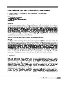
Figure 1: Average NRMSE for the MackeyGlass TS with fixed and evolved inputs NRMSE) with networks of similar sizes. However, the results are mixed, and to fully understand the benefits, or otherwise, of evolving the inputs, one needs to look more carefully at what emerges for the individual TS. Table 2 presents the number of evolved inputs found after 2000 generations (columns 2-5), the fixed number of inputs found with the False Nearest Neighbours method (column 6) and the delays found using the Average Mutual Information (column 7). Here is not presented the delays found with the evolutionary algorithm because many complex variations are possible. For example, if ten inputs are available {xt , ..., xt−9 }, three fixed inputs with a delay of 2 means using {xt , xt−2 , xt−4 }, but if the inputs are evolved, more complex selections could emerge, such as {xt , xt−5 , xt−7 } or {xt−4 , xt−7 , xt−8 }. A clear example of this issue arises with the Henon TS. Table 4 shows that the best evolved network in this case has 7 inputs, which are {xt , xt−1 , xt−3 , xt−5 , xt−9 , xt−15 , xt−16 }, in which the delays between inputs are unequal. If the inputs are fixed, the False Nearest Neighbour method gives a value of 5 and the Average Mutual Information gives a delay of 9 (Table 2), which corresponds to having the input vector {xt , xt−9 , xt−18 , xt−27 , xt−36 }. Even though there are more parameters to evolve if the inputs are not fixed, the algorithm can still obtain faster results in some cases. For example, in Fig. 1 is shown the average NRMSE over the entire evolution, with fixed and evolved inputs, for the Mackey-Glass TS. It can be seen that the evolution of inputs allows the algorithm to obtain smaller errors faster (particularly at the beginning of the evolution). Conversely, there were other cases where the error was reduced faster if the inputs were fixed, for example the QP2, QP3, Rossler, Star and D1 TS.
Table 2: Evolved inputs versus fixed inputs in the EPNet algorithm with 2000 generations Evolution of inputs
F ixed values
T ime Series M ean
Std Dev
M in
M ax
Inputs
Delays
Henon
10.23
2.800041
5
16
5
9
Ikeda
11.57
2.329471
6
16
7
5
Logistic
12.40
2.190890
7
16
3
9
Lorenz
12.63
2.189053
9
17
5
17
Mackey-Glass
12.47
1.995397
8
17
19
19
Qp2
12.67
1.625939
10
16
7
22
Qp3
11.63
1.629117
7
15
9
6
Rossler
11.10
1.936046
6
14
13
12
Births in Quebec
11.20
2.074475
5
14
21
4
Dow Jones
11.50
1.943158
8
16
21
46
Gold Prices
11.40
2.206573
8
16
21
27
IBM Stock
12.27
2.016028
6
17
19
52
SP500
12.07
2.273283
6
16
21
25
Colorado River
11.10
2.564344
5
16
13
3
Lake Eriel
11.13
2.255007
5
15
17
7
Equipment Temp. 11.17
2.780267
5
17
17
33
Kobe
11.83
2.290661
8
16
5
4
Star
13.10
2.171127
10
17
5
6
Sunspot
11.33
1.971055
7
16
19
23
D1
10.93
2.504249
6
15
21
8
Laser
13.10
1.647359
9
17
19
2
In Tables 3 and 4 are presented the NRMSE and network sizes for the fixed and evolved inputs respectively. It is these results that were summarized in Table 1. Columns 2-5 give the mean, standard deviation, minimum and maximum values of the NRMSE (evaluated on previously unseen test sets) for the best individuals from the 30 runs. Columns 6-8 give the number of inputs, hidden nodes and connections of the best individuals overall from the 30 runs, corresponding to the NRMSE in column M in. Comparing the results for individual TS, there are no obvious patterns indicating why evolved inputs provide better NRMSE performance in some cases but not others. Although evolving the inputs means more parameters to evolve, the EPNet algorithm still finds smaller architectures for some TS, though larger architectures are found for others. Moreover, there appears to be no correlation between the cases of improved performance and any of the other differences that emerge as a result of having evolved rather than fixed inputs. For example, if the size of an ANN is taken to be the total number of trainable connections, then out of the 11 TS improved at 0.05 level of significance for the NRMSE, only 6 TS obtain smaller architectures for the best individual
found than when the inputs are fixed (Connections columns in Tables 4 and 3). These TS are Mackey-Glass, Dow Jones, Gold Prices, Colorado River, Lake Eriel and Laser. For the 8 TS that were better if the inputs are fixed, only QP2, QP3 and IBM Stock had smaller architectures than if the inputs are evolved.
4
Conclusions
This paper studied the issue of feature selection for evolved ANNs. It presented a series of experiments to determine whether it is better, or not, to evolve the inputs when the EPNet algorithm is used for TS prediction tasks. This was done by comparing evolving the inputs against keeping them at fixed computed values throughout the evolutionary process. The fixed inputs were computed using the approaches employed in previous studies, namely False Nearest Neighbour for the number of inputs and Average Mutual Information for their delays. It was shown that evolving the inputs gave significantly better prediction results for 11 of the 21 TS studied, but in 6 cases was it better to keep the inputs fixed. For the remaining 4 TS there was no significant difference. This led to the conclusion that it is certainly not the
Table 3: Individual TS results for fixed inputs. Evolved NRMSE and architecture parameters for the best individual values over 30 runs with 2000 generations N RM SE
Best Ind.
T ime Series M ean
Std Dev
M in
M ax
Inputs
Hidden
Connections
Henon
0.785112
0.103130
0.552615
0.981666
5
14
131
Ikeda
0.959694
0.034274
0.849187
1.014560
7
14
144
Logistic
0.001052
0.000652
0.000217
0.002870
3
11
71
Lorenz
0.016993
0.009701
0.004919
0.047069
5
15
138
Mackey-Glass
0.336494
0.035695
0.259019
0.415552
19
10
176
Qp2
0.028665
0.006725
0.016584
0.043588
7
14
147
Qp3
0.176651
0.055778
0.093578
0.325843
9
12
128
Rossler
0.142443
0.247063
0.001809
1.118090
13
12
157 131
Births in Quebec
0.516288
0.029663
0.440343
0.586517
21
8
Dow Jones
1.409703
0.329013
0.744604
2.041210
21
9
178
Gold Prices
1.305383
0.415891
0.710825
2.427460
21
15
308
IBM Stock
0.715871
0.112638
0.459090
0.996211
19
12
200
SP500
0.597546
0.067702
0.444256
0.768787
21
15
288
Colorado River
0.964563
0.079263
0.844041
1.139390
13
15
223
Lake Eriel
0.770567
0.246672
0.425295
1.457200
17
9
140
Equipment Temp.
0.683046
0.173931
0.296670
1.207780
17
16
278
Kobe
1.009605
0.145755
0.668835
1.329590
5
16
153
Star
0.025598
0.004490
0.015847
0.036367
5
13
115
Sunspot
0.539722
0.110897
0.371779
0.897257
19
17
322
D1
1.030869
0.216930
0.569237
1.429940
21
14
272
Laser
0.153638
0.045795
0.088370
0.320004
19
14
268
Table 4: Individual TS results for evolved inputs. Evolved NRMSE and architecture parameters for the best individual values over 30 runs with 2000 generations N RM SE
Best Ind.
T ime Series M ean
Std Dev
M in
M ax
Inputs
Hidden
Connections
Henon
0.654182
0.197501
0.336084
1.038330
7
12
114
Ikeda
0.905389
0.061768
0.653851
0.991480
15
17
283 192
Logistic
0.000592
0.000378
0.000126
0.001495
12
15
Lorenz
0.019564
0.011186
0.003145
0.044841
17
16
290
Mackey-Glass
0.004186
0.002008
0.001673
0.012219
12
12
164
Qp2
0.071087
0.036165
0.025993
0.193532
13
17
258
Qp3
0.404328
0.120893
0.149107
0.630460
11
15
204
Rossler
0.005333
0.017721
0.000506
0.097060
11
17
242
Births in Quebec
0.513337
0.017996
0.465915
0.545526
12
19
306
Dow Jones
1.097907
0.053064
0.997859
1.211680
11
12
155
Gold Prices
1.057707
0.151929
0.835188
1.532440
14
14
205
IBM Stock
0.875539
0.062092
0.745606
0.995658
13
18
279
SP500
0.648791
0.025466
0.590659
0.706523
11
12
157
Colorado River
0.802570
0.090089
0.600033
0.968082
8
15
182
Lake Eriel
0.704184
0.103292
0.395519
0.920900
13
8
95
Equipment Temp.
0.784072
0.088246
0.604829
0.939192
11
13
157
Kobe
0.808204
0.145650
0.543781
1.166810
11
15
192
Star
0.022751
0.005533
0.013487
0.033852
17
14
245
Sunspot
0.670356
0.100118
0.446804
0.873600
10
9
93
D1
1.089576
0.216749
0.714094
1.525940
14
13
202
Laser
0.060268
0.018450
0.026656
0.091397
14
17
263
case that using the values given by the False Nearest Neighbour and Average Mutual Information is the best way to perform input feature selection, i.e. to fix the inputs during the evolutionary process. However, one can also conclude that the standard EPNet algorithm is not capable of finding the best input features in all cases either. Moreover, looking at the detailed results for individual TS did not reveal any clear picture of when evolving the inputs would be better. Since it should in principle be possible for the evolution of the inputs to find the computed inputs used in the fixed input case, one needs to ask why the EPNet algorithm is not finding them in the cases where they lead to better performance than the actual evolved inputs. One possibility is that the evolution simply needs to be run for even more generations, and that is something that clearly needs to be explored further. Another issue is that the mutation operations of adding or deleting random inputs introduce a lot of noise into the operation of the evolving ANNs, and for some TS that is clearly leading to worse performance than if the inputs are fixed. This suggests two more strands for taking this research further: first looking more carefully at the disruption caused by the changes to the inputs during evolution, and second looking at making the evolution of inputs easier by starting at the computed values so that evolution can improve on them where possible, but hopefully not end up with inferior values. By following these ideas it is hoped that simple extensions to the evolutionary ANN approach presented in this paper will result in improved feature selection and resultant performance in many cases, and worse performance in none.
Acknowledgments This research was supported by the University of Birmingham through the BlueBEAR cluster. The first author would like to thank CONACYT for the scholarship given for his graduate studies.
References [1] J. Belaire-Franch and D. Contreras. Recurrence plots in nonlinear time series analysis: Free software. Journal of Statistical Software, 7(9), 2002. [2] H. Braun and P. Zagorski. ENZO-M - A hybrid approach for optimizing neural networks by evolution and learning. In Parallel Problem Solving from Nature – PPSN III,
pages 440–451, Berlin, 1994. Springer. [3] M. Dash and H. Liu. Feature selection for classification. Intelligent Data Analysis, 1:131–156, 1997. [4] R. J. Frank, N. Davey, and S. Hunt. Time series prediction and neural networks. Journal of Intelligent and Robotic Systems, 31:91–103, 2001. [5] C.-L. Huang and C.-Y. Tsai. A hybrid SOFM-SVR with a filter-based feature selection for stock market forecasting. Expert Systems with Applications, 36(2, Part 1):1529–1539, 2009. [6] H. A. Mayer and R. Schwaiger. Evolutionary and coevolutionary approaches to time series prediction using generalized multi-layer perceptrons. Proceedings of the 1999 Congress on Evolutionary Computation, CEC 99, 1:275–280, 1999. [7] J. Mcdonnell and D. Waagen. Evolving recurrent perceptrons for time-series modeling. IEEE Transactions on Neural Networks, 5(1):24–38, 1994. [8] R. G. Pajares, J. M. Ben´ıtez, and G. S. Palmero. Feature selection for time series forecasting: A case study. Proceedings of the International Conference on Hybrid Intelligent Systems, pages 555–560, 2008. [9] H. Takenaga, S. Abe, M. Takatoo, M. Kayama, T. Kitamura, and Y. Okuyama. Optimal input selection of neural networks by sensitivity analysis and its application to image recognition. Proceedings of the MVA ’90. IAPR Workshop on Machine Vision Applications, 1990. [10] F. Takens. Detecting strange attractors in turbulence. In Dynamical Systems and Turbulence, Warwick 1980, volume 898, pages 366–381, Berlin, 1981. Springer. [11] X. Yao. Evolving artificial neural networks. Proceedings of the IEEE, 87(9):1423–1447, 1999. [12] X. Yao and Y. Liu. EPNet for chaotic timeseries prediction. In SEAL’96: Selected papers from the First Asia-Pacific Conference on Simulated Evolution and Learning, pages 146–156, London, UK, 1997. Springer-Verlag. [13] X. Yao and Y. Liu. A new evolutionary system for evolving artificial neural networks. IEEE Transactions on Neural Networks, 8(3):694–713, 1997. [14] H. Yoon and K. Yang. Feature subset selection and feature ranking for multivariate time series. IEEE Trans. on Knowledge and Data Engineering, 17(9):1186–1198, 2005.