Clustering Data Set with Categorical Feature Using Multi Objective Genetic Algorithm Dipankar Dutta
Paramartha Dutta
Jaya Sil
Department of Computer Science and Information Technology, University Institute of Technology, The University of Burdwan, Golapbug (North), Burdwan, West Bengal, India PIN-713104 Email:dipankar
[email protected]
Department of Computer and System Sciences, Visva-Bharati University, Santiniketan, West Bengal, India PIN-731235 Email:
[email protected]
Department of Computer Science and Technology, Bengal Engineering and Science University, Shibpur, West Bengal, India PIN-711103 Email:
[email protected]
Abstract—In the paper, real coded multi objective genetic algorithm based K-clustering method has been studied where K represents the number of clusters known apriori. The searching power of Genetic Algorithm (GA) is exploited to search for suitable clusters and cluster modes so that intra-cluster distance (Homogeneity, H) and inter-cluster distances (Separation, S) are simultaneously optimized. It is achieved by measuring H and S using Mod distance per feature metric, suitable for categorical features (attributes). We have selected 3 benchmark data sets from UCI Machine Learning Repository containing categorical features only. Here, K-modes is hybridized with GA to combine global searching capabilities of GA with local searching capabilities of K-modes. Considering context sensitivity, we have used a special crossover operator called “pairwise crossover” and “substitution”.
I. I NTRODUCTION Data mining is an interdisciplinary field of research applied to extract high level knowledge from real-world data sets [14]. Clustering happens to be one of the important data mining task. Clustering is an unsupervised learning process where class labels are not available at the training phase. GA is “search algorithms based on the dynamics of natural selection and natural genetics” [17]. Categories of GAs are simple GA (SGA) and multi objective GA (MOGA). When an optimization problem involves only one objective, the task of finding the best solution is a single objective optimization problem. However, in the real world, life appears to be quite complex. Most of the problems are consisting of more than one interdependent objective, which are to be minimized or maximized simultaneously. These types of problems are multi objective optimization problem [6]. The use of GAs in clustering is an attempt to exploit effectively the large search space usually associated with cluster analysis and better interactions among the features to form chromosomes. Clustering is to primarily identification of natural groups within a data set. Instances in the same groups are more similar compared with instances in different groups [22],
[30], [32]. From optimization viewpoint, clustering is a nondeterministic polynomial-time hard (NP-hard) grouping problem [12]. Evolutionary algorithms like GAs are metaheuristics widely believed to be effective on NP-hard problems, being able to provide near-optimal solutions to such problems in reasonable time. Although GAs have been used in data clustering problems,most of them are single objective in nature. Naturally, this is hardly equally applicable to all kinds of data sets. So to solve many real world problems like clustering, it is necessary to optimize more than one objective simultaneously by MOGA. As the relative importance of different clustering criteria are unknown, it is better to optimize Homogeneity (H) and Separation (S) separately rather than combining them into a single measure to be optimized. Objects within the same clusters are similar implying low intra-cluster distances (H) and at the same time, objects belonging to different clusters are dissimilar, thereby inducing high inter-cluster distances (S). In the paper, clustering is considered as an intrinsically multi objective optimization problem [22] by involving homogeneity and separation together. However, choosing optimization criterion is one of the fundamental dilemmas in clustering [33]. This paper is organized as follows. Section II reports previous relevant works. Section III clarifies definitions pertaining to the problem. Section IV describes the proposed approach for solving the problem. In section V, testing are carried out on some popular benchmark data sets. Finally, section VI summarizes the work with concluding remarks. II. P REVIOUS W ORK Clustering is one of the most studied areas of data mining research. Extensive surveys of the clustering problems and algorithms are presented in [15], [19], [26], [30], [46]. With the growing popularity of soft computing methods, researchers of late extensively use intelligent approaches in cluster analysis of data sets. The methods are broadly categorized as (i) Partitioning methods, (ii) Hierarchical methods, (iii) Density-based meth-
ods, (iv) Grid-based methods, (v) Model-based methods and (vi) Clustering by Genetic Algorithm (GA). Among these partitioning methods and GA based methods are relevant here. Partitioning methods: Data sets are divided among K many partitions or clusters where K ≤ m, and m is the number of objects or tuples in the data sets. In this category, most popular methods are K-means [37], [38], fuzzy C-means (FCM) [3], K-modes [27], [28], fuzzy K-modes [29] and K-medoids [32]. Among these K-means and FCM cannot be applied in categorical domains. K-modes and fuzzy K-modes are popular methods in this domain. Clustering by Genetic Algorithms: Initially GAs were used to deal with single objective optimization problems such as minimizing or maximizing a variable of a function. Such GAs is simple GA (SGA). David Schaffer proposed vector evaluated genetic algorithm [50], which was the first inspiration towards MOGA. Several improvements on the vector evaluated genetic algorithm are proposed in [17]. Vector evaluated genetic algorithm dealt with multivariate single objective optimization. V. Pareto suggested Pareto approach [45] to cope with multi-objective optimization problems. In this work, chromosomes lying on the Pareto optimal front (dominant chromosomes) are selected by MOGA, providing near optimal solutions for clustering. According to the dominance relation between two candidate chromosomes, a candidate clustering chromosome Ch1 dominates another candidate clustering chromosome Ch2 if and only if: 1) Ch1 is strictly better than Ch2 in at least one of all the measures considered in the fitness function and 2) Ch1 is not worse than Ch2 in any of the measures considered in the fitness function. Researchers developed different implementation of MOGA e. g. NPGA [25], SPGA [52], PAES [34], NSGA-II [7], CEMOGA [1]. In this paper, we have developed our own MOGA to find out near optimal clusters by optimizing H and S values. From the viewpoint of the chromosome encoding scheme MOGA can be categorized in binary coded MOGA and real coded MOGA. In order to keep the mapping between the actual cluster modes and the encoded modes effective, real coded MOGA has been implemented in the work. Traditional clustering algorithms often fail to detect meaningful clusters because most real-world data sets are characterized by a high-dimensional, inherently sparse data space [21]. However, most popular K-modes clustering algorithm [27], [28] applied on original data sets may converge to non-optimal values. To find a globally optimal clustering solution, GA has been used for clustering. Most of the clustering approaches, whether single objective or multi-objective, are converted to a single objective by weighed sum method [31] or by any other means. However, only a few MOGA clustering approaches have been proposed so far and their experimental results have demonstrated that MOGA clustering approaches significantly outperform existing single objective GA clustering approaches [20], [21]. Earlier work on clustering by the single objective genetic algorithm are [9], [13], [18], [39], [41], [44], [51] and by MOGA are [2], [8], [10], [16], [23], [35], [36], [40],
[42], [43], [47], [48], [49]. Among them, fuzzy clustering on categorical data has been applied in [8], [16], [40], [42], [43]. DB Index [5] has been used to compare performance of clustering algorithms. It shows the superiority of global optimization capability of GA over local search algorithm like K-modes. III. D EFINITIONS A relation R and a list of features A1 , A2 , ...An defines a relational schema R(A1 , A2 , ...An ), where n = total number of features. The domain of Ai is dom(Ai ), where 1 ≤ i ≤ n. X represents a data set comprising a set of tuples. That is X = {t1 , t2 , ...tm }, where m = total number of tuples or records. Each tuple t is an n-dimensional attribute vector, i.e., an ordered list of n values i.e. t = [v1t , v2t , ...vnt ], where vit ∈ dom(Ai ) , with 1 ≤ i ≤ n. vit is ith value in tuple t, which corresponds to feature Ai . Each tuple t belongs to a predefined class, represented by vnt where vnt ∈ dom(An ) and vnt or class t labels are not known. So, t = [v1t , v2t , ...vn−1 ]. Formally, the problem is stated as every ti of X (1 ≤ i ≤ m) is to be clustered into K number of non-overlapping groups {C1 , C2 , ...CK }; where C1 ∪ C2 ∪ ...CK = X, Ci ̸= Ø, and Ci ∩ Cj = Ø for i ̸= j and j ≤ K. The solution of the clustering problem is a set of Cluster Mode (CM) that is {CM1 , CM2 , ...CMK }. (n − 1)dimensional feature vector, that is [ci1 , ci2 , ...cin−1 ] represents CMi . Equations (1), (2) and (3) calculate Mod distance per feature between one cluster center and one tuple, two cluster centers and two tuples respectively. n−1 ∑
d(CMi , tj ) = [[
M OD(cil , vlj )]/(n − 1)]1/2
(1)
M OD(cil , cjl )]/(n − 1)]1/2
(2)
l=1 n−1 ∑
d(CMi , CMj ) = [[
l=1 n−1 ∑
d(ti , ij ) = [[
M OD(vli , vlj )]/(n − 1)]1/2
(3)
l=1
M OD(cil , vlj ), M OD(cil , cjl ) and M OD(vli , vlj ) are all equal to 0 if cil = vlj , cil = cjl and vli = vlj . Otherwise they are equal to 1. IV. P ROPOSED A PPROACHES Original data sets are rearranged to label the last feature as class label and so class label becomes the nth feature. In clustering, class labels are unknown so we are considering first (n − 1) features of data sets. A. MOGA (H, S) Flowchart of MOGA (H, S) is provided in figure 1 and described below.
Fig. 1.
Flowchart of MOGA (H, S)
1) Building initial population: In most of the literature on GA, fixed number of prospective solutions build initial population (IP). Here, the size of IP is the nearest integer value of 10% of total number of tuples (m) in the data set. Although correlation between IP size and the number of instances in the data set are not explicitly known, our experience suggests that IP size guides searching power of GA and therefore its size should increase with the size of the data set. K number of tuples are chosen randomly to constitute j th chromosome Chj where 1 ≤ j ≤ initial population size (IP S) in a population. The process is repeated for IP S number of times. Each chromosome represents a prospective solution, which is a set of cluster modes (CMs) of K clusters. As tuples of data set build cluster modes, it induces faster convergence of MOGA, compared to building chromosomes by randomly choosing categorical feature values from the same feature domain. 2) Reassign cluster modes: Using every chromosome, a set of CMs, represented as, {CM1 , CM2 , ...CMK } are randomly initialized. K-modes algorithm 1 produces a set of new clus∗ ter modes that is {CM1∗ , CM2∗ , ...CMK }, which forms new chromosomes.
3) Crossover: Chromosomes generated by K-modes algorithm are input to the crossover. Context insensitivity is an important issue in a grouping task like clustering. Meaning of context insensitivity is “the schemata defined on the genes of the simple chromosome do not convey useful information that could be exploited by the implicit sampling process carried out by a clustering GA” [12]. In their survey paper Hruschka et. al. [26] shows drawback of conventional single point crossover operators often described in the literature considering context sensitivity. We have used a special crossover operator called “Pairwise crossover” described by Fr¨ anti in [13] as “The clusters between the two solutions can be paired by searching the “nearest” cluster (in the solution B) for every cluster in the solution A. Crossover is then performed by taking one cluster centroid (by random choice) from each pair of clusters. In this way we try to avoid selecting similar cluster centroids from both parent solutions. The pairing is done in a greedy manner by taking for each cluster in A the nearest available cluster in B. A cluster that has been paired cannot be chosen again, thus the last cluster in A is paired with the only one left in B.” This algorithm does not give the optimal pairing (2-assignment) but it is a reasonably good heuristic for the crossover purpose. Crossover probability (Pco ), chosen as 0.9 that is 90% chromosomes undergo with this crossover. 4) Substitution: Substitution probability (Psb ) of MOGA is 0.1. Child chromosomes are produced by crossover are parent chromosomes of this step. Here dom(Ai ) is categorical. In conventional mutation, any random value from dom(Ai ) can replace vi resulting different chromosomes. Considering context sensitivity, instead of replacement of any vi of chromosome, substitution is replacing cluster modes by any tuples randomly. Approximately number of substitution (Nsb ) = ⌊(Npch × K × Psb )⌋. 5) Combination: At the end of every generation of MOGA some chromosomes are lying on the Pareto optimal front. These chromosomes have survived and these are known as Pareto chromosomes. Chromosomes obtained from previous substitution method (section IV-A4), say N Cpre and previous generation Pareto chromosomes (section IV-A8) of MOGA, say P Cpre are considered to perform in the next generation. For the first generation of GA, P Cpre is zero because of the nonexistence of previous generation. In general, for ith generation of MOGA, if N Cpre is m and P Cpre at the end of (i − 1)th generation of MOGA is n then after combination, number of chromosomes are n + m or P Cpre + N Cpre . 6) Eliminating duplication: Survived chromosomes from previous generation may be generated again in the present generation of MOGA, resulting multiple copies of the same chromosome. So in this step system is selecting unique chromosomes from the combined chromosome set. One may argue with the requirement of this step. But if we remove this step then population size will be very high at the end of some iterations of GA. 7) Fitness Computation: As stated earlier, intra-cluster distance (Homogeneity) (H) and inter-cluster distances (Separa-
tion) (S) are two measures for optimization. Maximization of 1/H and S are the twin objectives of MOGA. It converts the optimization problem befitting into max-max framework. The values of H and S are computed by using Mod distance per feature measures. Equation 1 is calculating Mod distance per feature between one cluster center and one tuple. If dlowest (CMi , tj ) is the lowest distance for any value of i (where 1 ≤ i ≤ K), then tj is assigned to Ci . Ties are resolved arbitrarily. Equation 4 defines Hi (average intracluster distance or homogeneity of ith cluster). m ∑ Hi = [ dlowest (CMi , tj )]/mi
(4)
j=1
where mi is the number of tuples belonging to ith cluster and tj is assigned to ith cluster based on lowest distance. Summation of Hi is H, defined in equation 5 as H=
K ∑
Hi
(5)
i=1
Say, tj and tp are two distinct tuples from a data set where tj is assigned to Cx and tp is assigned to Cy . S is defined in equation 6 using dlowest (CMi , tj ) as S=
m ∑
d(tj , tp )
(6)
j,p=1
where j ̸= p and x ̸= y. 8) Selection of Pareto chromosomes: All chromosomes lying on the front of max(1/H, S) are selected as Pareto chromosomes. The process is not restricting the number of selected chromosomes. In other words, maximizing 1/H and S are two objectives of MOGA. As this process is applied after combination, elitism [6], [7] is adhered to. 9) Building intermediate population: From 2nd generation onwards, for every even generation, selected Pareto chromosomes of previous generation build the population. This helps to build a population of chromosomes close to the Pareto optimal front resulting fast convergence of MOGA. For every odd generation of MOGA or if for any generation previous generation of MOGA does not produce Pareto chromosomes greater than 2 then population are generated using procedure discussed in section IV-A1. This introduces new chromosomes in population and induces diversity in the population. Population size also varies from generation to generation. From the above discussion, one may get wrong idea that we are destroying any search we are carrying out during a generation and there is no solution evolution. In other words, there is really no time for evolution. But notice that, we are preserving Pareto chromosomes at every generation (ith generation of GA) and that is combined to present generation chromosomes ((i+1)th generation of GA) during Combination (section IV-A5). Selection of Pareto chromosomes are done on combined population set (section IV-A8). As pointed out, that
at every odd generation we generate the population applying the same procedure through which the initial population (section IV-A1) was generated. But is these cases we are not loosing Pareto chromosomes selected by previous even generation because we stores them in a separate storage. V. T ESTING AND C OMPARISON K-modes is most popular partition based traditional clustering method [27], [28] for categorical attributes. Algorithm 1describes steps of the K-modes. Algorithm 1 Algorithm for K-modes 1: Choose K initial cluster modes {CM1 , CM2 , ...CMK } randomly from m tuples {t1 , t2 , ...tm } of X where t = t [v1t , v2t , ..., vn−1 ]. 2: Assign tuple tj , j = 1, 2, ...m to cluster Ci , i ∈ {1, 2, ...K} iff d(CMi , tj ) < d(CMp , tj ), p = 1, 2, ...K, and i ̸= p. /* Using equation 1 */ Resolve ties arbitrarily. ∗ 3: Compute new cluster modes {CM1∗ , CM2∗ , ...CMK } as follows: CMi∗ =Mode of tj where tj ∈ Ci and j = 1, 2, ...m. 4: If CMi∗ = CMi , i = 1, 2, ...K then stop. Otherwise repeat from step 2. Note that in case the process does not stop at step 4 normally, then it is carried out for a maximum fixed number of iterations. We have taken a maximum fixed number of 100 iterations, which is incidentally same as the number of generations of GA. It is observed that in most of the cases it stops much before maximum fixed number of iterations. In literature different validity indices are available to measure the quality of clusters. Davies-Bouldin (DB) Index [5] is used here. Equation 7 is calculating DB Index.
DB Index = 1/K
K ∑
max((Hi + Hj )/d(CCi , CCj ))
i=1,i̸=j
(7) where K is the number of clusters, Hi is the average distance of all patterns in cluster i to their cluster mode CMi , Hj is the average distance of all patterns in cluster j to their cluster mode CMj and d(CMi , CMj ) is the distance of cluster modes CMi and CMj . The performance of two clustering algorithms are compared on the basis of the results obtained out of the three popular data sets from UCI Machine Learning Repository [24]. Table I summarizes features of data sets. Table II compares results obtained by the two clustering algorithms. For every data set and for every clustering algorithm, average values of 10 individual runs are tabulated. As K-modes algorithm is dealing with only one solution A3 is equivalent to B3, B4, B5 of MOGA (H, S). Following important observations are summarized here, based on the analysis of table II. H for all data sets in column
TABLE II C OMPARISON
OF PERFORMANCE OF CLUSTERING ALGORITHMS
Meaning of notations used in this table A1:H of K-modes, A2:S of K-modes, A3:DB Index of K-modes B1:Optimized min. H of MOGA (H, S) population, B2:Optimized max. S of MOGA (H, S) population, B3:DB Index of chromosome giving optimized min. H of MOGA (H, S) population, B4:DB Index of chromosome giving optimized max. S of MOGA (H, S) population, B5:Average DB Index of MOGA (H, S) population, B6:Best DB Index of MOGA (H, S) population Methods Data set Soybean(Small) Tic Tac Toe Zoo
A1 0.49 0.98 0.61
K-modes A2 277.71 156334.57 1909.37
TABLE I F EATURES OF DATA SETS USED IN THIS ARTICLE (H ERE , # N UMBER OF ). Name Soybean(Small) Tic Tac Toe Zoo
#Tuples 47 958 101
#Attributes 35 9 18
A3 0.95 1.27 1.24
INDICATES
#Classes 4 2 7
B1 0.41 0.96 0.52
B2 289.43 157324.8 1957.21
MOGA (H, S) B3 B4 0.86 0.91 0.96 2.24 0.83 1.16
B5 0.87 1.43 1.093
B6 0.77 0.96 0.77
VI. C ONCLUSIONS In this work, we have implemented a novel real coded hybrid elitist MOGA for K-clustering (MOGA (H, S)). It is known that elitist model of GAs provides the optimal string as the number of iterations increases to infinity [4], [11]. We have achieved one important data mining task of clustering by finding cluster modes. We have considered only categorical features in this work. Continuous features need other type of encoding, as Mod distance per feature measures is not suitable for those types of features. Dealing with missing features values and unseen data are other problem areas. It may be interesting to adapt MOGA based K-clustering for categorical features with unknown number of clusters. Deciding optimum value of k is another research issue. Authors are working in these directions. R EFERENCES
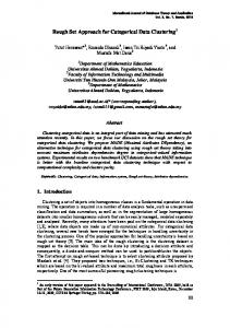
Fig. 2. H, S, Best DB Index of MOGA (H, S) population vs Generation of MOGA (H, S) for Soybean(Small) data set
B1 is lower than the values in column A1 because K-modes algorithm is doing local optimization or it locally optimizes intra cluster distance and MOGA (H, S) globally optimizes intra cluster distance. Result shows the superiority of GA over K-modes. Lowest DB Index of the population (column B6) of the proposed MOGA (H, S) is much better than DB Index obtained by K-modes (column A3). In the figure 2 we have plotted H, S and Best DB Index of MOGA (H, S) population vs Generation of MOGA (H, S) for a particular run with Soybean(Small) data set. Values of H and DB Index are varies in the range of 0 to 2. Values of S is varies from 288 to 290. We have converted it in the range of 0 to 2 before plotting. Due to the use of special population building process, hybridization of K-modes with GA, special crossover and substitution operator GAs are producing good clustering solution in a smaller number of iterations (100).
[1] S. Bandyopadhyay, S. K. Pal, and B. Aruna, “Multiobjective GAs, quantitative indices and pattern classification,” IEEE Trans. Syst., Man, Cybern.–B, vol. 34, no. 5, Oct. 2004, pp. 2088–2099, doi:10.1109/TSMCB.2004.834438. [2] S. Bandyopadhyay, U. Maulik, and A. Mukhopadhyay, “Multiobjective genetic clustering for pixel classification in remote sensing imagery,” IEEE Trans. Geosci. Remote Sens., vol. 45, no. 5, May. 2007, pp. 15061511, doi:10.1109/TGRS.2007.892604. [3] J. C. Bezdek, Pattern Recognition with Fuzzy Objective Function Algorithms. New York, NY: Plenum, 1981. [4] D. Bhandari, C. A. Murthy, and S. K. Pal, “Genetic algorithm with elitist model and its convergence,” Int. J. Patt. Recog. Art. Intel., vol. 10, no. 6, Jul. 1996, pp. 731–747, doi:10.1142/S0218001496000438. [5] D. L. Davies, and D. W. Bouldin, “A cluster separation measure,” IEEE Trans. Pattern Anal. Mach. Intell., vol. PAMI-1, no. 4, Apr. 1979, pp. 224-227, doi:10.1109/TPAMI.1979.4766909. [6] K. Deb, Multi-Objective Optimization Using Evolutionary Algorithms. New York: John Wiley & Sons, 2001. [7] K. Deb, A. Pratap, S. Agarwal, and T. Meyarivan, “A fast and elitist multiobjective genetic algorithm: NSGA-II,” IEEE Trans. Evol. Comput., vol. 6, no. 2, Apr. 2002, pp. 182-197, doi:10.1109/4235.996017. [8] S. Deng, Z. He, and X. Xu, “G-ANMI: A mutual information based genetic clustering algorithm for categorical data,” KnowledgeBased Systems, vol. 23, no. 2, Mar. 2010, pp. 144-149, doi:10.1016/j.knosys.2009.11.001. [9] K. Dhiraj, and S. K. Rath, “Comparison of SGA and RGA based clustering algorithm for pattern recognition,” Int. J. of Recent Trends in Engg., vol. 1, no. 1, May. 2009, pp. 269–273. [10] D. Dutta, P. Dutta, and J. Sil, “Clustering by multi objective genetic algorithm,” in Proc. of 1st Int. Conf. on Recent Advances in Information Technology (RAIT 2012), IEEE Press, Dhanbad, India, Mar. 2012, pp. 548–553, doi:10.1109/RAIT.2012.6194619.
[11] P. Dutta, and P. DuttaMajumder, “Convergence of an evolutionary algorithm,” in Proc. of the 4th Int. Conf. on Soft Computing (IIZUKA 1996), World Scientific, Fukuoka, Japan, Sep.–Oct. 1996, pp. 515–518. [12] E. Falkenauer, Genetic Algorithms and Grouping Problems. New York, NY: John Wiley & Sons, 1998. [13] P. Fr¨ anti, J. Kivij¨ arvi, T. Kaukoranta, and O. Nevalainen, “Genetic Algorithms for Large-Scale Clustering Problems, The Computer Journal, vol. 40, no. 9, Sep. 1997, pp. 547-554, doi:10.1093/comjnl/40.9.547. [14] A. A. Freitas, “A Survey of Evolutionary Algorithms for Data Mining and Knowledge Discovery,” in Advances in Evolutionary Computing of Natural Computing Series, Chapter 33, A. Ghose, and S. Tsutsui, Eds. Berlin, Heidelberg: Springer Berlin Heidelberg, 2003, pp. 819–845, doi:10.1007/978-3-642-18965-4 33. [15] K. Fukunaga, Introduction to Statistical Pattern Recognition. 2nd ed., New York, NY: Academic Press Prof., 1990. [16] G. Gan, J. Wu, and Z. Yang, “A genetic fuzzy K-Modes algorithm for clustering categorical data,” Expert Systems with Applications, vol. 36, no. 2, Mar. 2009, pp. 1615-1620, doi:10.1016/j.eswa.2007.11.045. [17] D. E. Goldberg, Genetic Algorithms for Search, Optimization, and Machine Learning. 1st ed., Reading, MA: Addison-Wesley Longman, 1989. ¨ [18] L. O. Hall, I. B. Ozyurt, and J. C. Bezdek, “Clustering with a genetically optimized approach,” IEEE Trans. Evol. Comput.. vol. 3, no. 2, Jul. 1999, pp. 103–112, doi:10.1109/4235.771164. [19] J. Han, and M. Kamber, Data Mining: Concepts and Techniques. San Francisco, CA, USA: Morgan Kaufmann, 2005. [20] J. Handl, and J. Knowles, “Evolutionary multiobjective clustering,” in Proc. 8th Int. Conf. Parallel Problem Solving From Nature (PPSN VIII), Birmingham, UK, 2004, pp. 1081–1091. X. Yao, E. K. Burke, J. A. Lozano, J. Smith, J. J. Merelo Guerv´os, J. A. Bullinaria, J. E. Rowe, P. Ti˜no, A. Kab´an, and H. Schwefel, Eds., in Lecture Notes in Computer Science, chapter 109, vol. 3242, pp. 1081–1091, Berlin, Heidelberg: Springer Berlin Heidelberg, 2004, doi:10.1007/978-3-540-30217-9 109. [21] J. Handl, and J. Knowles, “Exploiting the Trade-off - The Benefits of Multiple Objectives in Data Clustering,” in Proc. of 3rd Int. Conf. on Evolutionary Multi-Criterion Optimization (EMO 2005), Guanajuato, Mexico, 2005, pp. 547–560. C. A. Coello Coello, A. H. Aguirre, and E. ZitzlerEds., in Lecture Notes in Computer Science, chapter 38, vol. 3410, pp. 547–560, Berlin, Heidelberg: Springer Berlin Heidelberg, 2005, doi:10.1007/978-3-540-31880-4 38. [22] J. Handl, and J. Knowles, “Multi-objective clustering and cluster validation,” in Multi-objective Machine Learning, Y. Jin, Ed., in Studies in Computational Intelligence, chapter 2, vol. 16, pp. 21–48, Berlin, Heidelberg: Springer Berlin Heidelberg, 2006, doi:10.1007/3-540-330194 2. [23] J. Handl, and J. Knowles, “An evolutionary approach to multiobjective clustering,” IEEE Trans. Evol. Computat., vol. 11, no. 1, Feb. 2007, pp. 56-76, doi:10.1109/TEVC.2006.877146. [24] S. Hettich, C. Blake, and C. Merz, “UCI repository of machine learning databases,” 1998. [Online]. Available: http://www.ics.uci.edu/ mlearn/MLRepository.html [25] J. Horn, N. Nafploitis, and D. E. Goldberg, “A niched Pareto genetic algorithm for multiobjective optimization,” in Proc. IEEE Conf. Evolutionary Computation, IEEE press, Orlando, FL, USA, 1994, pp. 82–87, doi:10.1109/ICEC.1994.350037. [26] E. R. Hruschka, R. J. G. B. Campello, A. A. Freitas, and A. C. P. L. F. de Carvalho, “A survey of evolutionary algorithms for clustering,” IEEE Trans. Syst., Man, Cybern.–C, vol. 39, no. 2, Mar. 2009, pp. 133–155, doi:10.1109/TSMCC.2008.2007252. [27] Z. Huang, “Clustering large data sets with mixed numeric and categorical values,” in Proc. 1st Pac. Asia Knowl. Discovery Data Mining Conf., World Scientific, Singapore, 1997, pp. 21–34. [28] Z. Huang, “Extensions to the k-means algorithm for clustering large data sets with categorical values,” Data Mining Knowl. Discovery, vol. 2, no. 3, 1998, pp. 283-304. [29] Z. Huang, and M. K. Ng, “A fuzzy k-modes algorithm for clustering categorical data,” IEEE Trans. Fuzzy Syst., vol. 7, no. 4, Aug. 1999, pp. 446-452, doi:10.1109/91.784206. [30] A. K. Jain, M. N. Murty, and P. J. Flynn, “Data clustering: a review,” ACM Comput. Surveys., vol. 31, no. 3, Sep. 1999, pp. 264–323, doi:10.1145/331499.331504. [31] H. Jutler, “Liniejnaja modiel z nieskolmini celevymi funkcjami (linear model with several objective functions),” Ekonomika i Matematiceckije Metody, (In Polish), vol. 3, no. 3, pp. 397–406, 1967.
[32] L. Kaufman, and P. J. Rousseeuw, Finding Groups in Data: An Introduction to Cluster Analysis. New York: John Wiley & Sons, 1990. [33] J. Kleinberg, “An impossibility theorem for clustering,” in Advances in Neural Information Processing Systems, vol. 15, S. Becker, S. Thrum, and K. Obermayer, Eds., Cambridge, MA: MIT Press, 2002, pp. 446–453. [34] J. D. Knowles, and D. W. Corne, “Approximating the nondominated front using the Pareto archived evolution strategy,” Evol. Comput., vol. 8, no. 2, Jun. 2000, pp. 149–172, doi:10.1162/106365600568167. [35] E. E. Korkmaz, J. Du, R. Alhajj, and K. Barker, “Combining advantages of new chromosome representation scheme and multi-objective genetic algorithms for better clustering,” Intell. Data Anal., vol. 10, no. 2, Mar. 2006, pp. 163-182. [36] M. H. C. Law, A. P. Topchy, and A. K. Jain, “Multiobjective data clustering,” in Proc. IEEE Comput. Soc. Conf. on Comput. Vision and Pattern Recognit (CVPR 2004), vol. 2, IEEE press, Washington, DC, Jun.-Jul. 2004, pp. 424–430, doi:10.1109/CVPR.2004.1315194. [37] S. Lloyd, “Least squares quantization in PCM,” IEEE Trans Inform Theory, vol. 28, no. 2, Mar. 1982, pp. 129–137, doi: 10.1109/TIT.1982.1056489.(Original version: Technical Report, Bell Labs, 1957). [38] J. B. MacQueen, “Some methods for classification and analysis of multivariate observations,” in 5th Berkeley Symp. Math. Stat. Probability, Statistical Laboratory of the University of California, Berkeley, 1967, pages 281–297. [39] U. Maulik, and S. Bandyopadhyay, “Genetic algorithm-based clustering technique,” Pattern Recognit., vol. 33, no. 9, Sep. 2000, pp. 1455–1465. [40] U. Maulik, S. Bandyopadhyay, and I. Saha, “Integrating clustering and supervised learning for categorical data analysis,” IEEE Trans. Syst. Man. Cybern. A, vol. 40, no. 4, Jul. 2010, pp. 664-675, doi:10.1109/TSMCA.2010.2041225. [41] P. Merz, and A. Zell, “Clustering gene expression profiles with memetic algorithms,” in Proc. of the 7th Int. Conf. on Parallel Prob. Solving from Nature (PPSN VII)., Lecture Notes in Computer Science, chapter 78, vol. 2439. Berlin, Heidelberg: Springer Berlin Heidelberg, 2002, pp. 811-820, doi:10.1007/3-540-45712-7 78. [42] A. Mukhopadhyay, U. Maulik, and S. Bandyopadhyay, “Multiobjective genetic fuzzy clustering of categorical attributes,” in Proc. 10th Int. Conf. on Inf. Technol. (ICIT 2007), IEEE press, Orissa, India, Dec. 2007, pp. 74-79, doi:10.1109/ICIT.2007.13. [43] A. Mukhopadhyay, U. Maulik and S. Bandyopadhyay, “Multiobjective genetic algorithm-based fuzzy clustering of categorical attributes,” IEEE Trans. Evol. Computat., vol. 13, no. 5, Oct. 2009, pp. 991–1005, doi:10.1109/TEVC.2009.2012163. [44] H. Pan, J. Zhu, and D. Han, “Genetic algorithms applied to multi-class clustering for gene expression data,” Genomics, Proteomics, Bioinformatics, vol. 1, no. 4, Nov. 2003, pp. 279–287. [45] V. Pareto, Manuale di Economia Politica. Milan:Piccola Biblioteca Scientifica, 1906. Translated into English by A. S. Schwier, and A. N. Page, Manual of Political Economy, London:Kelley Publishers, 1971. [46] L. Parsons, E. Haque, and H. Liu, “Subspace clustering for high dimensional data, a review,” SIGKDD Explor. Newsl., vol. 6, no. 1, Jun. 2004, pp. 90–105, doi:10.1145/1007730.1007731. [47] K. S. N. Ripon, C. H. Tsang, and S. Kwong, “Multi-objective data clustering using variable-length real jumping genes genetic algorithm and local search method,” in Proc. of Int. Joint Conf. on Neural Networks (ICJNN 2006), IEEE press, Vancouver, BC, 2006, pp. 3609–3616, doi:10.1109/IJCNN.2006.247372. [48] K. S. N. Ripon, C. H. Tsang, S. Kwong, and M. Ip, “Multi-objective evolutionary clustering using variable-length real jumping genes genetic algorithm,” in Proc. of 18th Int. Conf. on Pattern Recognition, Hong Kong, Aug. 2006, pp. 1200–1203, doi:10.1109/ICPR.2006.827. [49] K. S. N. Ripon, and M. N. H. Siddique, “Evolutionary multi-objective clustering for overlapping clusters detection,” in Proc. of the 11th Conf. on Congress on Evolutionary Computation (CEC 2009), IEEE Press, Piscataway, NJ, May. 2009, pp. 976–982, doi:10.1109/CEC.2009.4983051. [50] J. D. Schaffer, “Multiple objective optimization with vector evaluated genetic algorithms,” in Proc. 1st Int. Conf. Genetic Algorithms, L. Erlbaum Associates, Pittsburgh, PA, Jul. 1985, pp. 93–100. [51] P. Scheunders, “A genetic c-means clustering algorithm applied to color image quantization,” Pattern Recognition, vol. 30, no. 6, Jun. 1997, pp. 859-866, doi:10.1016/S0031-3203(96)00131-8. [52] E. Zitzler, “Evolutionary Algorithms for Multiobjective Optimization: Methods and Applications,” Ph.D. dissertation, Swiss Federal Institute of Technology (ETH), Zurich, Switzerland, 1999.