and Infrastructure Management of the U. S. Department of Energy under. Contract No. ..... The use of sampling technique in large databases have been used for ...
Clustering High Dimensional Massive Scientific Datasets* Ekow J. Otoo and Arie Shoshani Lnwrence Berkeley National Lnboratory 1 Cyclotron Road University of California Berkeley, CA 94720
Seung-won Hwang Dept. of Computer Science University of Illinois at Urbana-Champaign 1304 M! Springfield Ave. Urbana, IL 61801
Abstract
Clustering algorithms for multidimensional datasets have general applications in content-based retrieval of multimedia objects, i.e., images, text, digital videos, etc. Of equal significance are their applications in scientific data management. Not only can they be used for storing related data in close proximity to each other to aid query processing, but they also provide a pre-analysis categorization of the dataset for further scientific investigation. For example the use of clustering methods, to group objects from physics experiments with the purpose of optimizing data access and computations, is discussed in [7, 81. Most of the clustering algorithms proposed so far are impractical in handling extremely large datasets that have very high dimensionality. Our work on clustering is motivated by the quest for algorithms that can group scientific data for efficient query processing. Examples of such datasets are those generated by experiments conducted in High Energy Physics (HEP) [9, 11, 101. Results of these experiments generate or are expected to generate data of the order 10" - 1015 bytes that would reside on tape robots. Large disk farms, of the order of tens to hundreds of Terabytes, would act as disk caches to support jobs that would run on large CPU farms. The goal of clustering in this setting, is to optimize I/O performance under changing access patterns so that near sequential reading can be achieved for all queries. A generalization of the problem without restricting it to any specific application domain is as follows. Given a set of bounded ordered domains Ao,AI, . . ., AM-^, that are not necessarily distinct, let SM = A0 x A1 x .. . x AM-1 be an M-dimensional feature space. A domain Aj may be either numeric or categorical. Let R = { T O , r l , . . .,T N - ~ } be a set of objects (or records), where each object is defined as an M-dimensional feature vector. That is, an object ri = (a,,o,ai,l.. . a i , ~ - l ) where , ai,j E A j . Each object corresponds to a point (i.e., an "image point" of the object), in the multidimensional feature space S M .The objective of clustering is to partition the N points into subgroups, called clusters, according to some similarity measure ciq(ri,r j ) , under the metric n o m L,. For some specified distance E
Many scientific applications can benejit from eficient clustering algorithm of massively large high dimensional datasets. However most of the developed ,algorithms are impractical to use when the amount of data is very large. Given N objects each de3ned by an M-dimensional feature vectol; any clustering techniquefor handling very large datasets in high dimensional space should run in time O ( N )at best, and O ( N log N ) in the worst case, using no more than O ( N M )storage,for it to be practical. A parallelized version of the same algorithm should achieve a linear speed-up in processing time with increasing number of processors. We introduce a hybrid algorithm called HyCeltyc, as an approachfox clustering massively large high dimensional datasets. HyCeltyc, which stands for Hybrid Cell Density Clustering method, combines a cell-density based algorithm with a hierarchical agglomerative method to identiJL clusters in linear time. The main steps of the algorithm involve sampling, dimensionality reduction and selection of signijicantfeatures on which to cluster the data.
1. Introduction Clustering is the act of grouping objects characterized by feature vectors (or attribute vectors) into classes, such that pairs of objects within the same class are similar according to some defined similarity measure. Pairs of object from different classes are dissimilar under the same measure. Clustering algorithms have had wide applications in pattern recognition, image processing, statistical data analysis and recently in data mining and knowledge discovery. 'This work is supported by the Director, Office of Laboratory Policy and Infrastructure Management of the U. S. Department of Energy under Contract No. DE-AC03-76SF00098. This research used resources of the National Energy Research Scientific Computing (NERSC), which is supported by the Office of Science of the U.S. Department of Energy.
147 U.S. Govemment Work Not Protected by U.S. Copyright
x
image points in SM become very sparse and highly skewed. Second, the choice of the bin sizes not only determines the quality of the clusters identified but also determines the space and time complexity of the algorithm. Third, since the number of grid cells could be very much larger than even the number of points, we require a data structure for managing only the non-empty cells. Our approach is to find a solution to these problem by using a hybrid of methods. We refer to this scheme as HyCeltyc which stands for Hybrid Cell Density Clustering method. To address the first problem, i.e. the effect of large dimensionality. we apply a linear dimensionality reduction method called FastMap [3], on a sample of the data to reduce the dimensionality from M to K , where K is the desired dimensionality for clustering. In addition to the resulting reduced dimensionality,we developed a method to order the dimensions according to their ability to discriminate the clusters. To address the second problem of selecting the bin sizes; we specify as an input to the algorithm, a threshold value 73. The value of il defines the minimum number of points in a cell that allows it to be considered as dense. This value of 71,expressed either as an absolute value-or as a percentage of the number of points, is also utilized to determine the bin sizes of each attribute. This is explained in detail in'section 3. The third problem is resolved by hashing the addresses of non-empty cells to a linear address space. The literature gives a well defined classification of the different clustering algorithm. These include partirioning, hierarchical-agglomerative, hierarchical-divisive, densitybased and grid-based methods. A grid-based method would be appropriately referred to as cell-based method. A taxonomy of the different clustering methods is given in [12]. The HyCeZfyc clustering scheme we proposed. in this paper is a hybrid of the cell-based, the density-based, and the hierarchical-agglomerative clustering method. The detailsof these techniques are explained in the subsequent sections. HyCeltyc executes in six phases. Let S M denote the M dimensional attribute space and let S K denote the attribute space in K-dimensions for K < M . The six,phases of the algorithm are:
an object ri belongs to the same cluster as the object r j if the nearest neighbor of ri is r j and b q ( r j , r j ) 5 E . The two objects r j , r j are said to be similar (or near) to each other. Otherwise they belong to different clusters and are dissimilar (or farther apart) from each other. A cluster may be depicted as a dense region of objects and can be of any arbitrary shape. The application domain determines the choice of the domains Aj's, how the feature vector of each object is characterized and what distance measure to use. For the purposes of our applications, we consider the attributes to be numeric and more specifically they are interval-scaled. An intervalscaled variable is a continuous measurement of near linear scale such as length, weight, energy level, etc. Of main concern is the fact that we have to deal with very large feature space having tens to hundreds of dimensions and very large number of objects of the order of millions and possibly billions. Although numerous clustering algorithmshave been proposed and studied extensively in the past [4, 121, most of these proposed methods are impractical to use on the scale of data being considered. The major limitations are that some methods require all the data to be in memory, e.g. BIRCH [26], while others require a priory knowledge of the number of clusters, e.g.. K-Means [12, 141. 0thers rely on dimensionality reduction techniques that usually involve Singular Value Decomposition (SVD), Discrete' Fourier Transforms (DFI'), Karhunen-Loeve and MultiDimensional Scaling (MDS). These have either quadratic, and sometimes cubic, complexity in the number of objects N, or in the number ofdimensions M. The. most effi'cientmethods for large datasets are the socalled "grid-based" algorithms, but they all have some deficiencies that we will explain below. They typically require a single pass over the datilwhich can be disk resident); to generate counts of the number of objects per cell. Find-.' i n i the clusters has a complexity proportional to the number of populated cells which is a lot smaller than the number'of cells. 'Examples of such methods are: MAFIA [ 161. STING [25], and Celtyc [23]. We chose to use Celtyc because of its ability to form clusters based on detecting "valleys" between clusters (see [23] for details). The essential cluster generation steps of these methods involve two principal ideas; a partitioning of the feature-space into cells and determining maximal connected regions of dense-cells. We will refer.to such connected regions as dense regions. The cells are rectilinearly. prirtitioned subspaces of the featurespace where each feature or attribute defines an axis. The interval of values of each attribute Aj is split into mj bins. The number of cells generated, which is denoted as T, is M-1 given by K = &=, mj. ' f i e grid-based algorithms, while efficient, all suffer from the following three problems. First, for 'large M , the
i) Sampling from the-original,.data$et.. , ii) Dimensionality reduction fr0m.M t o - K based on the , . sample drawn. I
.
iii) Cell-density clustering of the sample in the reduced K . dimensional space S K . I
.
.
.
.
iv) Refinement of the clusters mapped onto the original M-dimensional space, S;..
i
v) Selection of K significant features out of the original ' M features of the origirial feature space;
148
vi) Cell-density clustering of the entire dataset based on the significant attributes identified in phase (v); Although the refinement step in HyCeltyc computes distances between objects, the computation is restricted to pairs of objects within the same dense region. The algorithms therefore executes in time O ( K N ) using O(NM) space. The main contribution of this paper is that by using a combination of algorithms we succeeded in developing a method for clustering high dimensional massively large dataset that runs in linear time and in linear space. The technique being advocated establishes a general framework for clustering high dimensional massive datasets. The rest of the paper is organized as follows. In the next section we summarize some of the closely related works to our scheme. We then describe the details of the various steps of the algorithms used in each phase of HyCeltyc in section 3. The complete HyCeltyc algorithm is formally presented in section 4. A short analysis of the proposed method is presented in section 5 and we conclude with section 6.
Object
A0
A1
A2
P
0.31
Q
0.10 0.11 0.58 0.50
17.8 9.30 21.5 22.0 16.0
3.0 3.0 1.0 2.0 1.0
R S T
Table 2 . l a : Sample Dataset
Object P
Q
P 0.79 0.58 0.69 0.61
R S
T
R
Q
S
T
1.0 0.75
1.0
1.0
1.0
0.36
1.0
0.17 0.34
0.15 0.72
Table 2 . l b : Similarity Matrix
Hierarchical clustering begins by determining the largest value in the similarity matrix. Note that this is obtained during the similarity matrix computation. Examination of the Table 2.lb reveals that objects P and Q are closest. The rows and columns corresponding to the two points P and Q are removed and the similarity matrix is updated with the set {P,Q} considered as a single cluster. To update the matrix, the distance between a point p and a cluster may be computed either a$the distance between p and a point q, within the cluster that is closest to p or between p and the point q that is furthest from p . The former measure gives what is referred to as the single-link method. The latter measure gives what is referred to as the complete-link method. One could utilized the average distance between p and all points in the cluster as a measure of closeness. In this case we get the average-link method. If we update the similarity matrix according to the single-link measure, we get the Table 2.2a below.
2. Related Works
x
A number of clustering algorithms have been proposed and extensively studied in the literature [123. One class of widely used clustering algorithms are the hierarchical methods. We adopt a variant of the hierarchical method generally referred to as a hierarchical-agglomerative clustering.
2.1. Hierarchical Agglomerative Clustering To carry out hierarchical clustering, one begins by defining a similarity function between pairs of objects and then constructing a Similarity Matrix. This is usually given by the normalized Euclidean distances between pairs of objects. The Euclidean distance between a pair of objects, T, = (a,,o,a,,l.. . ~ , , M - I ) and T q = (aq,o,a4,1. . . a q ,- 1~) is given by
T
Obiect PQ
P.0 1.0
R
R S
0.58 0.69
1.0 0.51
1.0
T
0.61
0.72
0.75
S
1.0
Table 2.2a: First Updated Similarity Matrix
j=O
Each distance is then converted into a similarity value by the equation 2:
Object
P,Q
P.Q R
1.o
R
S,T
0.58 1.0 S,T 0.61 0.72 1.0 Table 2.26: Second Updared Similarity Matrix
where amaxis the distance between the two farthest pair and
P,Q 1.0
R,S,T
RQ R,S.T
0.69
1.0
Object
c,,~ always lies between 0 and 1. For example, suppose we have 5 objects with 3 attributes Ao, A I ,Az as shown in Table 2.la and the Similarity Matrix is as given by Table 2.lb.
Table 3: Final Updated Similarity Matrix
149
z j = 0,1,. . . ,mj
- 1. Consequently each cell of the partitioned space is uniquely identified by the M-dimensional index (x0,zl. . .ZM-I). where xj is the integer number associated with the interval [ Z j , z j , ~ j , ~The ~ number ) . of cells generated by such partitioning is given by K = mj . A record ri is assigned to a cell C M ( z O21,. , . . , ~ M - I )if . for its feature vector (ai,o,ui,l .. . u i , ~ - l )Z ,j , z j 5 ui,j < ~ j , , ~ j ,= {0,1,. . .M - 1) for zj = {0,1,. . . mj - 1). The differences in the various methods concern:
0.0
0.2
n';:
0.4
0.6
-
1.0
1 How the cells are maintained. For example BIRCH uses a tree structure called a clustering feature tree very much like a B-tree to store information on nonempty cells, DBSCAN uses an R* - tree, STING uses multilevel quadtree-like structure, GridClus uses a Grid-File and DENCLUE uses a B+-tree.
1 P
O
R
S
T
Figure 1: Single-Link Dendogram
The iterative process of merging points to the nearest clusters finally gives Table 3. The result of such a hierarchical clustering is often depicted as a dendogram that is shown in Figure 1. The computation of similarity function for very large dataset would be quite involved and as such we utilize this only in a refinement step when we generate clusters of the sample dataset. The main computation in HyCeltyc is done as a cell-density based clustering algorithm.
2 What information is stored within the cells. In this respect, BIRCH stores summary statistics such as moments while STING maintains statistical informations such as means, standard deviation, min, max, etc.
2.2. Density Based Clustering
4 The method used for dimensionality reduction if any.
3 The algorithm used to merge connected dense regions.
5 Whether projecting cluster onto lower dimensional feature space is used to determine the significant features to carry out clustering.
Efficient clustering methods that are appropriate for very large or high dimensionality are generally cell-density ba$ed. These include BIRCH [26] (Balanced Iterative Reducing and Clustering using Hierarchies), CLARANS (Clustering Large Applications based on R4Ndomized
6 Whether clustering is done on the entire dataset or on repeated selected samples.
Search) [20] and DBSCAN (Density-based Spatial Clus-
A summary of the various methods can be found in [12,
tering of Applications with Noise) [151. Closely related works that utilize elements of hierarchical grid-density and projected clustering method include CLIQUE (CLustering in QUEst) [19], DENCLUE (Clustering Based on Density Distributions) [5], GridClus(GRID-CLUStering) [211, MAFIA [ 161, OptiGrid (OPTImal GRID-Clustering) [61, STING (STatistical INformation Grid-based) 1251 and Wavecluster (WAVElet-based CLUSTERing) [22]. Of these, only MAFIA has demonstrated a parallelization of its algorithm called pMAFIA, on a shared nothing multiprocessor system. The basic idea of the cell-density and grid-based clustering algorithms is the partitioning of the feature space. The feature space SM is quantized rectilinearly into nonoverlapping rectangular subspaces called cells. Suppose each attribute Aj is defined by the range of values [ L j ,V j ] . The range of values is partitioned into bins of equal intervals [Zj,zj,uj,zj),so that each bin spans Ij,zj= IAj(/mj values, where mj is the number of bins into which the attribute Aj is split. Each attribute Aj is an ordered domain also referred to as interval-scaled. Hence the intervals Ij,z may be progressively ordered in increasing integer values
41. A summary of the time and space complexity of the
different schemes is shown in Table 4, using the parameters defined below for measuring the clustering algorithms.
N : Number of data points.
M : Dimensionality of original data space.
mj: Number of bins into which attribute j is partitioned. N,: Sample size drawn from the dataset, N , z,: Number of clusters in a sample, z,