Clustering on Dynamic Social Network Data Pascal Held1 and Kai Dannies1 Abstract This paper presents a reference data set along with a labeling for graph clustering algorithms, especially for those handling dynamic graph data. We implemented a modification of Iterative Conductance Cutting and a spectral clustering. As base data set we used a filtered part of the Enron corpus. Different cluster measurements, as intra-cluster density, inter-cluster sparseness, and Q-Modularity were calculated on the results of the clustering to be able to compare results from other algorithms. Key words: clustering, graph clustering, stream data, cluster measurements, enron data set
1 Introduction Social network analysis has already been popular long before websites like Facebook, XING or Google+ - now commonly known as social networks were launched. In [16] a comprehensive approach of modeling social network data as (un)directed graphs was proposed, which has become widely accepted. Over the years a lot of research has been performed on e.g. cohesiveness of groups of members in social graphs [17] or segmentation of social networks [13]. All these methods have in common that they use a static representation of the social graph underlying the respective social network. Recent research covered also the topic of dynamic graph clustering. Kim et al.[11] tried to solve the problem of clustering dynamic social networks by using evolutionary algorithms. Goerke et al.[8] extended an algorithm based on min-cut trees [6] introducing temporal smoothness. Attempts have been made to infer information from dynamic graphs (e.g. in [1]) but they either restrict themselves to fairly simple questions like connectivity or to path finding problems in order to cope with the changing structure of the graph. Such discretization results from some kind of binning operation performed on the data, thus leading to a loss of information, namely the exact time when an event has happened. Such an approach does not take into account the frequency with which events occur but rather lists their absolute number. We provide a reference clustering along with a prepared data set, bases on the Enron corpus. One can download them at http://www.ovgu.de/pheld/ pub/SMPS2012. The clustering we provide for each time step of the data Otto von Guericke University of Magdeburg,
[email protected] ·
[email protected]
Faculty
of
Computer
Science
1
2
Pascal Held and Kai Dannies
set is described in Section 2.1, a divisive minimum modularity clustering, generates very well clusters with respect to cluster measurements as intercluster sparseness or intra-cluster density. The paper is structured as follows: The following section gives a short summary of the Enron dataset and of the selected algorithms for clustering. Afterwards we present our experiments in Section 3 and the results in Section 4. We finish our paper with a conclusion in Section 5.
2 Foundations 2.1 Enron Dataset We used the well-known Enron dataset (http://www-2.cs.cmu.edu/~enron/) as basis for our experiments. The Enron dataset is a large corpus of email messages from the Enron Corporation. This email communication is a good example for human interaction in social networks. The raw dataset contains about 620, 000 messages from 158 users [12]. For our experiments we cleaned the messages, so we removed duplicate messages, and all messages, which were not sent from one Enron employee to another. Mails from mailing lists were also dropped. The major part of the dropped messages was SPAM and duplicated messages. We interpreted mails with multiple recipients as a separate mail from the sender to every recipient. Mails with wrong addresses, like
[email protected] were matched to the correct
[email protected]. From these messages we created an event list containing only the time stamps, the sender, and the recipient of the message. In total we got 9071 events. We used this event list to generate a dynamic graph, where every node is an Enron employee and every edge represents the communication frequency. The event list was binned to buckets of 10.000 seconds. In total we got about 10.000 of these time steps. To estimate this frequency we used a Butterworth filter with a bandpass-frequency of 0.0075. This value is the result of an optimization process, based on AIC and BIC measures. It is a good compromise between fast reaction on changing in behavior and smooth filter signal. A detailed description why we use this frequency can be found in [9]. A more detailed discussion about the resulting data set can be found at http://www.ovgu.de/pheld/pub/SMPS2012 The Enron dataset is not a really huge dataset, but this gives us the opportunity to cluster the resulting dynamic graph at a lot of time stamps with classical clustering methods. Later, the results of these classical algorithms can be compared with the results of dynamic clustering algorithms. Good results on this small datasets could be a indicator for good results in much larger datasets.
Clustering on Dynamic Social Network Data
3
2.2 Clustering Algorithms Graph clustering has obviously a close connection to the classical minimum cut problem [2], which consists in finding for a given (undirected) graph a partition of its vertices into two disjoint subsets, which minimizes the number (or the total weight) of the edges crossing between them. More precisely we try to find more than one cut here, but a “good” number of cuts for dividing the graph in the “most natural” way. Two values of the graph are important to determine the quality of the clustering: The number of edges between the clusters and the number of edges in each cluster. In section 2.3 we will present in detail several possibilities to combine those values to a single number as a quality measure of graph clustering. 2.2.1 Divisivel Minimum Modularity Clustering (DMMC) The basic idea of this algorithm is the same as in Iterative Conductance Cutting[10]. These algorithm aims for a cut of the graph minimizing the conductance, see section 2.3. Unfortunately finding such a cut is NP-hard. So Kannan et al.[10] used an approximation: the nodes are sorted w.r.t. their corresponding eigenvalues of the adjacency matrix. Then calculate each possible split of this sorted set and continue with the maximal conductance. We decided to use the recently deeply researched measurement of Modularity [3] as described in section 2.3. Besides this we decided because of the need of as good results as possible to actually solve the NP-hard problem: To try any possible cut to minimize the modularity. Even solving this problem does not guarantee an optimal solution with respect to modularity as measurement: There could be steps where a split in more than two clusters leads to a better result. So for really finding the best cluster we would have to check any possible clustering. Because this is computationally too extensive even for the given 158 nodes we hope to get a really good approximation by using the algorithm described below. As initialization we perform a connected component analysis. After this we perform a split on each cluster by taking each pair of nodes as seeds for the subsequent clusters and assigning all other nodes to the nearest cluster center. We keep, with respect to the Q-Modularity, the best split if its better then the original, unsplitted cluster. This is processed recursively on each cluster until none of the resulting cluster is split. 2.2.2 Other Algorithms As second algorithm we implemented the unnormalized spectral clustering as described by Luxburg[14] and compared it with DMMC. There are also other algorithms described in the literature. One example is Markov Clustering [5] that is simulating a random walk on the graph.
4
Pascal Held and Kai Dannies
Another one is Geometric MST1 Clustering [7] which combines spectral partitioning and a geometric clustering technique. Another prominent example is a clustering based on min-cut trees developed by Flake et al.[6].
2.3 Cluster Quality Measurements As stated above, two values of a graph clustering are especially important to measure the quality of a clustering: The sum of the weights of intra-cluster edges should be maximized and the sum of the weights of inter-cluster edges should be minimized. Because one wants only one number to compare clusterings, different measurements based one those two numbers were developed [2, 4]. In this section we will use following notation: |E| sum of weights of edges contained in E E(C) intra-cluster edges of Cluster C E(C1 , C2 ) inter-cluster edges between C1 and C2 Einc (C) incident edges to a cluster, including inter-cluster edges from C to any other cluster as well as all intra-cluster edges of C maxWeight for simple, undirected graphs with 0 ≤ edgeWeight ≤ 1: | V | · | V − 1 | · 0.5 Q-Modularity The Q-Modularity measurement was developed by Newman und Girvan [15]. One sets up a k × k-Matrix M where k is the number of clusters. The entry (i, j) of the matrix is the sum of the edge weights between the i-th and the j-th cluster for i 6= j and the sum of weights of the i-th cluster for i = j. The Matrix is normalized by | M |. If this matrix has most of its weight on the principal diagonal then most of the weights are within clusters instead between the clusters and therefore the clustering is good. However, only using the elements on the principal diagonal to measure the cluster quality is not sufficient, because then singleton clusters would always be optimal. So the authors [15] choose the following quantity for taking the intercluster edges into account: ai =
X j
Mi,j =
| Einc (Ci ) | maxGraphWeight
The complete measurement is then calculated by: X Q-Modularity = (Mi,i − a2i ) i 1
MST = minimum spanning tree
(1)
(2)
Clustering on Dynamic Social Network Data
5
Intra-Cluster Density and Inter-Cluster Sparseness The basic idea of the intra-cluster density is to measure how dense the clusters are. For the intra-cluster density we used:
intraClusterDensity =
1 · numClusters
X C∈clusters
| E(C) | maxWeight(C)
(3)
The basic idea for this measurement is, that the edges between the clusters should be as sparse as possible. For inter-cluster sparseness we used: P | (u, v) | interClusterSparseness = 1 −
(u,v)∈E,u∈Ci ,v∈Cj ,i6=j
maxGraphWeight −
P
| E(C) |
(4)
C∈clusters
3 Experiments As stated above we used the Enron dataset for our experiments. The results achieved by processing the raw data as described in Section 2.1 lead to edge weights between zero and one, mostly much closer to zero. There are also different types of people. Some people communicate 100 times as much as other people, but they have also regularity in their communication behavior. The edge weights are approximately lognormal distributed, so we used a logarithmic scaling: 20 + log10 edgeWeight (5) 20 Numbers smaller than zero or greater than one were set to zero or one respectively. The number 20 is used as a threshold: All values above 10−20 shall be considered. Any threshold you want to use can replace this threshold. The higher this number is chosen the longer clustering structure from inactive users keep alive. Isolated nodes were ignored for the clustering. After this preprocessing we took every time step of the data and clustered it with DMMC and spectral clustering where the maximal number of clusters for the second algorithm was set to 25 because more than 25 clusters on 158 nodes are hard to interpret. For the spectral clustering we stored the best result out of 100 experiments to neglect the random component as good as possible. As the target function for both algorithms we maximized the QModularity. The other described measurements were used to compare the results independent of the target function, see next section. scaledEdgeWeight =
6
Pascal Held and Kai Dannies
4 Results In Figure 1 we show the generated number of clusters over the time. The x-axis describes the timeline, where 10.000 seconds are one time step. Both algorithms generated a similar number of clusters. The DMMC algorithm is more stable than the spectral clustering algorithm in terms of number of clusters. This is caused by on the random component in the K-Means used by the spectral clustering. This phenomenon is also reflected in the QModularity. Good values for the Q-Modularity are between 0.3 and 0.7 [15]. These values were reached by the DMMC algorithm most of the time. The DMMC algorithm outperforms the spectral clustering with the Q-Modularity measurement in each time step.
Fig. 1 left: number of clusters, right: Q-Modularity over time
The inter-cluster-sparseness, see Figure 2, is quite good for both algorithms. For this measurement the spectral clustering provides better results than the DMMC algorithm. There are some outliers at the beginning of the timeline. This results from less active elements in the graph at the first few hundred time steps. So each new event has a big influence on the resulting graph. However the DMMC algorithm provides better results for the intra-cluster density. This leads to the conclusion that DMMC prefers the intra-cluster density, but spectral clustering prefers the inter cluster sparseness. The lower values at the end of the time series are caused by the high connectivity of the graph.
5 Conclusion and Further Work We clustered the Enron corpus with two different clustering algorithms: Divisive Minimum Modularity Clustering and the spectral clustering. We evaluated the results of the algorithm with respect to three different clustering quality measurements: The intra-cluster density, the inter-cluster sparseness and the Q-Modularity. The DMMC algorithm is more stable over the time
Clustering on Dynamic Social Network Data
7
Fig. 2 inter-cluster-sparseness and intra-cluster-density over time
steps of the data due to the missing random component compared to spectral clustering. However, the disadvantage of DMMC is the much higher computation time. Both algorithms lead to reasonable results, though. Despite the long computation time, the DMMC can be used as reference to test other cluster algorithms. The results are suitable even if we haven’t tested all possible clusterings to find the real optimum for a given target function, we tried due to the construction of the algorithm a lot of possibilities and should always result in a quite good optimum. The comparison with the well known spectral clustering confirms this assumption. For future work one should test the described algorithms with other common stream data sets. Also the change of the clusterings in a small time range should be considered as measurement for clustering stream data. Another open question is, how similar are the clusterings of successive time steps. As a next step we will study how the clusters develop over time and how temporal smooth they really are. One main problem in social network clustering is, that there is no correct labeling for clusters available. In this paper we enriched a given dataset with such labels. It should be studied if our used measurements lead to good clustering results for social networks.
References [1] Alberts D, Cattaneo G, Italiano GF (1997) An empirical study of dynamic graph algorithms. J Exp Algoritm 2 [2] Brandes U, Gaertler M, Wagner D (2003) Experiments on graph clustering algorithms. In: Di Battista G, Zwick U (eds) Algorithms - ESA 2003, Lecture Notes in Computer Science, vol 2832, Springer Berlin / Heidelberg, pp 568–579
8
Pascal Held and Kai Dannies
[3] Brandes U, Delling D, Gaertler M, Goerke R, Hoefer M, Nikoloski Z, Wagner D (2008) On modularity clustering. IEEE Transactions on Knowledge and Data Engineering pp 172–188 [4] Delling D, Gaertler M, G¨orke R, Nikoloski Z, Wagner D (2006) How to evaluate clustering techniques. Interner Bericht Fakult¨at f¨ ur Informatik, Universit¨ at Karlsruhe; 2006, 24 [5] van Dongen SM (2001) Graph clustering by flow simulation. PhD thesis, University Utrecht [6] Flake GW, Tarjan RE, Tsioutsiouliklis K (2004) Graph clustering and minimum cut trees. Internet Mathematics pp 385–408 [7] Gaertler M (2002) Clustering with spectral methods. Master’s thesis, University Konstanz [8] Goerke R, Hartmann T, Wagner D (2009) Dynamic graph clustering using minimum-cut trees. Lecture Notes in Computer Science 5664:339– 350 [9] Held P, Moewes C, Braune C, Kruse R, Sabel BA (2012) Towards Advanced Data Analysis by Combining Soft Computing and Statistics, chap Advanced Analysis of Dynamic Graphs in Social and Neural Networks, pp 205–222 [10] Kannan R, Vempala S, Vetta A (2004) On clustering: Good, bad and spectral. Journal of the ACM (JACM) 51 [11] Kim K, McKay R, Moon BR (2010) Multiobjective evolutionary algorithms for dynamic social network clustering. Proceedings of the 12th annual conference on Genetic and evolutionary computation pp 1179– 1186 [12] Klimt B, Yang Y (2004) The enron corpus: A new dataset for email classification research. In: Boulicaut JF, Esposito F, Giannotti F, Pedreschi D (eds) Machine Learning: ECML 2004, Lecture Notes in Computer Science, vol 3201, Springer Berlin / Heidelberg, pp 217–226 [13] Kumar R, Novak J, Tomkins A (2006) Structure and evolution of online social networks. In: Proceedings of the 12th ACM SIGKDD international conference on Knowledge discovery and data mining, ACM, New York, NY, USA, KDD ’06, pp 611–617 [14] von Luxburg U (2007) A tutorial on spectral clustering. Statistics and Computing 17:395–416 [15] Newman MEJ, Girvan M (2004) Finding and evaluating community structure in networks. Phys Rev E 69:026,113 [16] Wassermann S, Faust K (1997) Social Network Analysis: Methods and Applications, Stuctural Analysis in the Social Sciences, vol 8. Cambridge University Press, Cambridge, UK [17] White DR, Harary F (2001) The cohesiveness of blocks in social networks: Node connectivity and conditional density. Sociol Methodol 31(1):305–359