Clustering Ordinal Survey Data in a Highly Structured Ranking Priy Werrij
Rianne Kaptein
Vrije Universiteit Amsterdam, The Netherlands
Crunchr Amsterdam, The Netherlands
Crunchr Amsterdam, The Netherlands
[email protected]
[email protected]
[email protected]
ABSTRACT In this paper we investigate how to cluster ordinal survey data in a highly structured ranking to identify groups of like-minded people. We experiment with several rank correlation coefficients to compare rankings, including Spearman’s rank-order coefficient and Kendall’s tau. To cluster the survey answers we use K-Means, spectral clustering and an evolutionary algorithm. K-Means clustering using Spearman’s rank-order coefficient with inverted tie-correct scores highest, but all results seem to lead to clusters with no significant cohesion.
1.
INTRODUCTION
Labeling people is something we all tend to do. In surveys, this often means that respondents are grouped by some chosen attribute in order to observe or investigate certain differences in their responses. However, for businesses it might be valuable to automatically detect groups of like-minded people. In other words: performing unsupervised clustering on the responses while excluding personal (demographic) data. Detecting groups in the data can help businesses to establish the appropriate strategies to satisfy their employees and/or clients. In this study we use survey responses that are gathered using the survey tool shown in figure 1. Respondents rank items in a diamond shape. The ordinal data itself has many tied ranks and is highly correlated: if one item is ranked highest (i.e. ‘most important’), others cannot have this rank anymore. Although the scale unit (i.e. importance), and size of the diamond are customizable, most conducted surveys are about importance of aspects in collective labor agreements. Often, survey data is ranked data in which respondents have to rank certain items or subjects on a certain scale. Few studies have been carried out on clustering ranked data. Moreover, most of these studies focused on describing the structure or analyzing the distribution of the ranks of all data together instead of assuming disagreement within the
Figure 1: Diamond shape in survey tool.
population [4]. While some even say that ranked (or ordinal) data is not appropriate for cluster analysis [8], Heiser and D’Ambrosio [4] reports on some studies which have succeeded to do so. These, and similar studies mostly use complex probabilistic models. However, Heiser and D’Ambrosio [4] implements a generalized K-means method and concludes that “loss-function based methods enjoy general advantages compared to methods based on probability models”. Other attempts of using classical cluster methods or loss-function based methods on clustering ranked data are not common. The aim of this study is to investigate how we can cluster ordinal survey data in a highly structured ranking. We answer the following two research questions: 1. How can we create rank correlation coefficients that accurately represent dissimilarity between survey responses? 2. How can we cluster ordinal survey data and allocate respondents into a pre-determined number of groups? We will experiment with several cluster techniques.
ACM ISBN 0-12345-67-8/90/01. DOI: 10.1145/1235
This paper is organized as follows. In the next section we find rank correlation coefficients to compare responses
(2)and compare the rank coefficients in terms of desirable behavior. In Section 3 we describe the clustering algorithms. In Section 4 we describe our experiments and evaluate the different sets of clusters. And finally, in Section 5 we draw our conclusions. This paper is a short version of Werrij [10].
2.
RANK CORRELATION COEFFICIENTS
A few rank correlation coefficients are available: for non normally distributed data the suggested coefficients are Spearman’s rank-order and Kendall’s tau rank correlation [3]. Both aforementioned coefficients range from -1 to 1, in which 0 suggests no correlation, -1 indicates that the ranks of a pair of responses are correlated negatively and 1 indicates that these are correlated positively [11].
Spearman’s rank-order coefficient Spearman’s rank-order coefficient uses the summed squared difference of item’s ranks to calculate the similarity [11]. This summed squared difference is then divided by a term based on the number of total items to make sure it is -1 when this difference is maximized and 1 if the difference is 0. Because it uses the difference of ranks, even the smallest differences in rank are penalized. It handles tied ranks by a correction of the divisor term. On top of that, it also sets values to the mean of the ranks of their positions in the ordered data set [11].
Kendall’s tau rank correlation Kendall’s tau rank correlation is based on the total number of discordant pairs of items in their ranking order [1]. Instead of using the exact ranks of items, it compares per item how many concordant and discordant pairs (in terms of ranking) there are and divides these by the total number of possible pairs. So although item’s ranks might be different for two responses, if many items are still ranked lower than others in both, the coefficient might still suggest a high correlation. The coefficient handles tied ranks only by a correction of the divisor term.
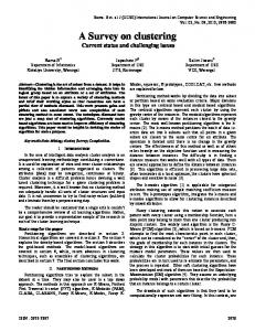
Spearman’s rank-order coefficient with inverted tie-correct The fact that Spearman’s rank-order coefficient handles ties by setting values to the mean of the ranks might not suffice for our use-case. We can see this in a small example, presented in figure 2, which uses a diamond shape with 5 levels to rank items in.
(a) Regular tie-correct
(b) Inverted tie-correct
Figure 3: Example of two kinds of tie-corrected ranks for Spearman’s rank-order coefficient
Spearman’s rank-order coefficient in which the tied ranks are corrected by using the centrally inverted differences (diffs) of the regular tie-correct mechanism. In the example: the regular tie-correct mechanism has [1.5, 2.5, 2.5, 1.5] as diffs between each of the possible ranks. Inverting this both ways from the center gives us [2.5, 1.5, 1.5, 2.5]. If we apply these diffs to our ranks, we get the tiecorrected ranks seen in figure 3b. By using this as basis for Spearman’s rank-order coefficient, the squared differences of item’s ranks will be larger for changes in top/bottom ranks.
2.1
Rank coefficient criteria
Before we use the introduced coefficients in the cluster algorithms, we evaluate them by comparing some responses. Particularly of interest was to verify whether the newly introduced Spearman’s rank coefficient with inverted tie-correct did what was expected of it. In consultation with domain experts a set of rough criteria was defined. The criteria consist of the desirable behavior of rank coefficients when faced with certain changes of ranks as follows: 1. For similar responses the rank coefficient should deviate very little. 2. For inverted responses the rank coefficient should be negative for fully inverted responses and neutral for centrally inverted responses. 3. For shifted responses the rank coefficient should be strongly positive for 1-rank shifts and positive for 2rank shifts. 4. For swapped responses the rank coefficient should deviate more for top/bottom item swaps than middle item swaps.
Figure 2: Example diamond shape with ranks When we correct these ranks for the ties, we get the values in figure 3a. As visible, the rank differences between more important items is in this case smaller than the difference between neutrally ranked items in the middle. One could argue that a swap of two items near the middle should not be the cause of a significant difference in coefficient. Therefore, we define another rank correlation coefficient based on
For every rank coefficient it was checked whether they were met sufficiently. As the criteria are rough guidelines, the fact whether the coefficients behaved sufficiently was decided on their relative behavior. Besides giving insights in their reaction to differences in responses it might also help in confirming what coefficient performs best. The criteria were checked by comparing a default response to several other responses by using the three rank coefficients. In these comparisons artificial responses for the (most common) 16 slot diamond were used. From our tests we conclude they all meet the first three criteria. For the fourth criteria, the swapped responses criteria, we find some differences so we look at it in more detail here.
Table 2: Description of the evolutionary algorithm
Consider the following three assignments of ranks to some items:
Representation Recombination Mutation
A := [1, 2, 2, 3, 3, 3, 4, 4, 4, 4, 5, 5, 5, 6, 6, 7] B := [2, 1, 2, 3, 3, 3, 4, 4, 4, 4, 5, 5, 5, 6, 7, 6] C := [1, 2, 2, 3, 3, 4, 3, 4, 4, 5, 4, 5, 5, 6, 6, 7]
Parent selection Survival selection Initialisation
Table 1: Swapped responses rank coefficients r
r(A, B) r(A, C)
Kendall tau 0.9434 0.8774
Spearman 0.9864 0.9258
Spearman inverted 0.9258 0.9864
(k) Centroid-based permutations Cycle crossover Non-uniform rank shift with adaptive step size Rank-based selection (µ + λ) selection Random
‘nearest’ other cluster, then the fitness function is defined as: f itness(i) =
The results in Table 1 show that when swapping top/bottom (r(A, B)) ranks both Kendall’s tau and Spearman’s rank coefficient reported a higher correlation compared to swapping middle ranks (r(A, C)). Only Spearman’s rank with inverted tie-correct has the desirable opposite behavior to deviate more for top/bottom item swaps than middle item swaps. Spearman’s rank coefficient with inverted tie-correct never exhibits unwanted behavior and sometimes results in more desirable results than the other rank coefficients. Consequently, we assume that this measure generates the best results when using it in the cluster algorithms.
3.
CLUSTERING
The rank correlation coefficients described in the previous sections can be used to determine the distance between two ranks. The cluster algorithms described in this section use these rank correlation coefficients to cluster survey responses into groups.
3.1
Popular Algorithms
Cluster methods come in many shapes and sizes. Two of the most popular ones are K-means and spectral clustering [2, 6, 9]. Both the spectral clustering and K-means algorithm are implemented using the scikit-learn library1 in Python in such a way that they can deal with any dissimilarity measure.
3.2
Evolutionary Algorithms
Many studies have shown that evolutionary algorithms for clustering problems prove to be superior compared to traditional algorithms [5, 6]. On top of that, the central ranking problem, in which finding an average ranking for a set of responses is the objective, can also be avoided by constructing an algorithm which has a set of clusters as representation. In other words: even if some clustering techniques create clusters with a strong structure, there are still many ways in which these can be represented as actual response. The implemented evolutionary algorithm follows the description in Table 2.
Fitness function To make the algorithm more efficient, the distance from a response (i) to a cluster is calculated not by averaging the dissimilarities of all its responses, but by taking the dissimilarity (d) to the real-valued representation of the cluster. Consider a to be the currently assigned cluster and b the 1
http://scikit-learn.org/
4.
d(b, i) − d(a, i) max{d(a, i), d(b, i)}
(1)
EXPERIMENTS
In this section we describe the data used, and the set-up and results of our experiments.
4.1
Data
We use survey data from six companies having 113, 149, 350, 493, 2451 and 3426 respondents. All surveys held were using the 16-slot diamond shape. Five of the surveys are about the importance of aspects for a collective labor agreement and one is about the competences which should be present in a certain department.
4.2
Set-up
To compare different kinds of cluster techniques, dissimilarity measures, cluster sizes and surveys, a script was created which would run any kind of a combination of these. Each combination was run three times and the script output the average calculation time, average (silhouette) score and a silhouette coefficient plot for the last run. In total there were 3 (cluster sizes) * 6 (surveys) * 3 (dissimilarity measures) * 3 (algorithms) = 162 averaged test cases. As the business requirement usually is to create up to a maximum of a handful of clusters, only benchmarks were run to compare 2, 3 and 4 number of clusters. Although the cohesion of clusters might be better with a larger number of clusters, from the business perspective it was more valuable to invest time on comparing the different techniques on a low number of clusters. To evaluate the sets of created clusters, we use the silhouette coefficient which is based on the cohesion and separation of each individual element (i.e. survey response) [7].
4.3
Results
Clustering results for 3 and 4 clusters are shown in Table 3 and 4 respectively. Due to space constraints we omit the results for cluster size 2. Results are similar to the results of cluster sizes 3 and 4. Also the results for Kendall’s tau coefficient are omitted, these always score lowest.
4.3.1
Dissimilarity measure
In all cases, using Kendall’s tau coefficient scored lowest, while in 61% of the 54 cases, using Spearman’s rank-order coefficient with inverted tie-correct scored highest. If we only look at the K-Means method cases, then in almost 80% the adapted Spearman’s rank-order coefficient scored best.
Table 3: Average silhouette scores for 3 clusters
Size 113 149 350 493 2,451 3,426
K-Means Sp. Sp.Inv 0.1724 0.1785 0.1579 0.1621 0.1781 0.1717 0.1416 0.1821 0.1487 0.1834 0.1316 0.1394
4.3.2
Clustering
Spectral Sp. Sp.Inv 0.1741 0.1704 0.1403 0.1374 0.1452 0.1510 0.1094 0.1275 0.1392 0.1730 0.1214 0.0998
Evolutionary Sp. Sp.Inv 0.1612 0.1767 0.1569 0.1561 0.1271 0.1648 0.1697 0.1789 0.1570 0.1481 0.1254 0.1403
Not only in cases in which the K-means scored best (highest silhouette score) was the number of negative silhouette coefficients low, but also in some test cases where other techniques scored better. In those cases, the other algorithms made the ‘sacrifice’ of having a cluster with some negative silhouette coefficients in order to reach a higher (average) silhouette score. Another observation is that the evolutionary algorithm often presented solutions in which the cluster sizes were not as equal as the other techniques. It seems that the algorithm often converged to solutions near the constraint boundary that cluster sizes for a solution should not be too imbalanced. All results generated seem to lead to clusters with no significant cohesion according to Rousseeuw’s proposed interpretations of the silhouette score.
4.3.3
Calculation time
The test cases of the benchmark were run on multiple computers, so exact calculation time varies. Therefore a relative comparison between cluster techniques and dissimilarity measures is more appropriate. All computation times were averaged by the number of responses of the survey. In the case of creating 2 clusters, if the K-means method’s average duration is 1, Spectral clustering is on average 2.5 times as slow and the evolutionary algorithm’s duration is on average 20 times longer.
5.
CONCLUSION
Our main goal was to examine whether it is possible to create meaningful clusters of ordinal survey data in a highly structured ranking. First we answered the research question: How can we create rank correlation coefficients that accurately represent dissimilarity between clusters?. Our custom Spearman’s rank-order coefficient with inverted tie-correct performs best for this specific data. Our second research question was: How can we cluster ordinal survey data and allocate respondents into a pre-determined number of groups? Taking into account performance and computation time, KMeans relatively does the best job. The combination of Kmeans and Spearman’s rank with inverted tie-correct leads to the best results. However, all of the silhouette scores suggest that clusters without significant structure were created, confirming the claim that this kind of data is unsuitable for cluster analysis [8]. On the contrary, it could also be the case that the conducted surveys do not have any distinguishable groups in them, or that more meaningful clusters could be created with larger, for the business less useful, k. Future research should consider optimizing the parameters of the evolutionary algorithm more for the specific data.
Table 4: Average silhouette scores for 4 clusters
Size 113 149 350 493 2,451 3,426
K-Means Sp. Sp.Inv 0.1699 0.1885 0.1607 0.1397 0.1572 0.1542 0.1280 0.1472 0.1378 0.1574 0.1186 0.1273
Spectral Sp. Sp.Inv 0.1636 0.1772 0.1242 0.1066 0.1327 0.1366 0.0831 0.1207 0.1146 0.1460 0.1038 0.0920
Evolutionary Sp. Sp.Inv 0.1626 0.1600 0.1370 0.1241 0.1247 0.1306 0.1293 0.1429 0.1180 0.1215 0.1185 0.1119
Also, it might be possible to create more meaningful clusters when some elements are left out. Some aspects of a collective labor agreement might not be related to the ranking of the other aspects, so excluding it from the calculation might improve the results. However, this would require specific analyses for each survey.
References [1] H. Abdi. Kendall rank correlation. In Neil Salkind, editor, Encyclopedia of Measurement and Statistics, pages 508–510. SAGE, Thousand Oaks (CA), 2007. [2] Zhu. C, F. Wen, and J. Sun. A rank-order distance based clustering algorithm for face tagging. In Computer Vision and Pattern Recognition (CVPR), pages 481–488, Providence (RI), June 2011. IEEE. [3] N.S. Chok. Pearson’s versus spearman’s and kendall’s correlation coefficients for continuous data. Master thesis, University of Pittsburgh, Graduate School of Public Health, 2008. [4] W.J. Heiser and A. D’Ambrosio. Clustering and prediction of rankings within a kemeny distance framework. In Algorithms from and for Nature and Life, pages 19– 31. Springer, 2013. [5] E.R. Hruschka, R.J.G.B. Campello, Freitas A.A., and A.C.P.L.F. De Varvalho. A survey of evolutionary algorithms for clustering. IEEE Transaction on System, Man, and Cybernetics, Part C (Applications and Reviews), 39(2):133–155, 2009. [6] U. Maulik and S. Bandyopadhyay. Genetic algorithmbased clustering technique. Pattern Recognition, 33: 1455–1465, 2000. [7] D.W. Rousseeuw. Silhouettes: a graphical aid to interpretation and validation of cluster analysis. Journal of Computational and Applied Mathematics, 20:53–65, 1987. R [8] SAS/STAT 9.22 User’s Guide. SAS Institute Inc., Cary, North Carolina, 2010.
[9] U. Von Luxburg. A tutorial on spectral clustering. Technical Report TR-149, Max Planck Institue for Biological Cybernetics, March 2007. [10] P. Werrij. Clustering ordinal survey data in a highly structured ranking. Research paper BA, Vrije Universiteit Amsterdam, July 2016. [11] J.H. Zar. Spearman rank correlation. In Encyclopedia of Biostatistics. John Wiley & Sons, Ltd, 2005.