Clustering repeated ordinal data: Model based ...

Clustering repeated ordinal data: Model based approaches using finite mixtures

by

Roy Ken Costilla Monteagudo

A thesis submitted to the Victoria University of Wellington in fulfilment of the requirements for the degree of Doctor of Philosophy in Statistics. Victoria University of Wellington 2017

Abstract Model-based approaches to cluster continuous and cross-sectional data are abundant and well established. In contrast to that, equivalent approaches for repeated ordinal data are less common and an active area of research. In this dissertation, we propose several models to cluster repeated ordinal data using finite mixtures. In doing so, we explore several ways of incorporating the correlation due to the repeated measurements while taking into account the ordinal nature of the data. In particular, we extend the Proportional Odds model to incorporate latent random effects and latent transitional terms. These two ways of incorporating the correlation are also known as parameter and data dependent models in the time-series literature. In contrast to most of the existing literature, our aim is classification and not parameter estimation. This is, to provide flexible and parsimonious ways to estimate latent populations and classification probabilities for repeated ordinal data. We estimate the models using Frequentist (Expectation-Maximization algorithm) and Bayesian (Markov Chain Monte Carlo) inference methods and compare advantages and disadvantages of both approaches with simulated and real datasets. In order to compare models, we use several information criteria: AIC, BIC, DIC and WAIC, as well as a Bayesian NonParametric approach (Dirichlet Process Mixtures). With regards to the applications, we illustrate the models using self-reported health status in Australia (poor to excellent), life satisfaction in New Zealand (completely agree to completely disagree) and agreement with a reference genome of infant gut bacteria (equal, segregating and variant) from baby stool samples.

ii

iii

Acknowledgments To write a PhD dissertation is like building a house from scratch. You need to draw the plans, choose the land, build the foundations and so on. It is a long and complex process but also a hugely rewarding one, once you see the house completed. Of course, you need the help of others to carry out such a mammoth endeavour. Many thanks to my advisors Ivy Liu and Richard Arnold for their unconditional support over nearly four years. I would have not been able to do it without you. Sincere thanks also to Shirley Pledger, Daniel Fernández, Petros Hadjicostas, Patricia Huambachano, and Peter Donelan from the School of Mathematics and Statistics for your advice, encouragment and friendship in this journey. ¨ I am also very grateful to my informal advisors: Peter Muller from University of Texas-Austin, Joseph Bulbulia from Victoria University of Wellington, Dean Hyslop from Motu and Russell Millar from University of Auckland. I feel very fortunate to have had your advice and mentorship over the different stages of my PhD. A special mention to Miles Benton from Queensland University of Technology and Aaron Darling from University of Technology Sydney for our conversations about Genomics (and baby poo). Last but not least, I would like to acknowledge John Hinde, Lynn Hunt and Laura Dumitrescu who reviewed this dissertation and provided many insightful comments and words of encouragment. Needless to say, all remaining errors and omissions are my responsability. I want to dedicate my doctoral dissertation to my family: my mum Lucia, my dad Valerio, and my brother Ronny in Peru; my partner Emma, ´ Valentino who is and our son Amaru in New Zealand; and our son Jesus flying around everywhere.

iv

Contents 1

Literature Review

1

1.1

Introduction . . . . . . . . . . . . . . . . . . . . . . . . . . . .

1

1.2

Models for Ordinal Data . . . . . . . . . . . . . . . . . . . . .

3

1.3

Models for repeated ordinal data . . . . . . . . . . . . . . . .

8

1.4

Model based clustering analysis for ordinal data . . . . . . .

12

1.5

Model based clustering for repeated ordinal data . . . . . . .

14

1.5.1

Parameter dependent models . . . . . . . . . . . . . .

14

1.5.2

Data dependent models . . . . . . . . . . . . . . . . .

17

Thesis Roadmap . . . . . . . . . . . . . . . . . . . . . . . . . .

19

1.6 2

Data

21

2.1

Life Satisfaction (NZAVS) . . . . . . . . . . . . . . . . . . . .

21

2.2

Health Satisfaction (HILDA) . . . . . . . . . . . . . . . . . . .

26

2.3

Infant gut bacteria (Metagenomics) . . . . . . . . . . . . . . .

29

I Frequentist Estimation

33

3

Proportional Odds Model

35

3.1

The Model . . . . . . . . . . . . . . . . . . . . . . . . . . . . .

35

3.2

Frequentist Estimation . . . . . . . . . . . . . . . . . . . . . .

43

3.3

Simulations . . . . . . . . . . . . . . . . . . . . . . . . . . . .

47

3.4

Model selection . . . . . . . . . . . . . . . . . . . . . . . . . .

56

3.5

Application: 2009-2013 Life Satisfaction in New Zealand . .

63

v

CONTENTS

vi 4

Trend Odds Model

75

4.1

Model . . . . . . . . . . . . . . . . . . . . . . . . . . . . . . . .

75

4.2

Model selection . . . . . . . . . . . . . . . . . . . . . . . . . .

80

4.3

Simulations . . . . . . . . . . . . . . . . . . . . . . . . . . . .

80

4.4

Case Study: Comparing POM and the TOM using HILDA data . . . . . . . . . . . . . . . . . . . . . . . . . . . . . . . . .

84

II Bayesian Estimation

89

5 Parameter dependent models

91

5.1

Latent random effects models: random walk by cluster . . .

91

5.2

Bayesian Estimation . . . . . . . . . . . . . . . . . . . . . . .

92

5.3

Construction of the MCMC chain . . . . . . . . . . . . . . . .

95

5.3.1

Proposals . . . . . . . . . . . . . . . . . . . . . . . . .

96

5.3.2

Acceptance Probabilities (Metropolis-Hastings ratio)

97

5.3.3

MCMC Convergence . . . . . . . . . . . . . . . . . . .

99

5.4

Model comparison . . . . . . . . . . . . . . . . . . . . . . . . 100

5.5

Simulations . . . . . . . . . . . . . . . . . . . . . . . . . . . . 102

5.6

5.7

5.5.1

Model comparison . . . . . . . . . . . . . . . . . . . . 107

5.5.2

Estimating a model with misspecified random effects 107

Case Study: 2009-2013 life satisfaction in New Zealand . . . 110 5.6.1


5.6.2

Parameter estimates . . . . . . . . . . . . . . . . . . . 114

5.6.3

Classification results . . . . . . . . . . . . . . . . . . . 114

Case Study: Variant strains in infant gut bacteria . . . . . . . 118 5.7.1


5.7.2

Parameter estimates . . . . . . . . . . . . . . . . . . . 122

6 Data dependent models

129

6.1

Latent transitional models . . . . . . . . . . . . . . . . . . . . 129

6.2

Model . . . . . . . . . . . . . . . . . . . . . . . . . . . . . . . . 130

CONTENTS

6.3 6.4 7

8

vii

6.2.1 Likelihood . . . . . . . . . . . . . . . . . . . . . . . . . 131 6.2.2 Bayesian Estimation . . . . . . . . . . . . . . . . . . . 131 6.2.3 MCMC Convergence . . . . . . . . . . . . . . . . . . . 133 6.2.4 Model Comparison . . . . . . . . . . . . . . . . . . . . 134 Simulations . . . . . . . . . . . . . . . . . . . . . . . . . . . . 135 Case Study: 2001-2011 self reported health status from HILDA139

Bayesian Non-Parametric models 7.1 Introduction . . . . . . . . . . . . . . . . . . . . . . . . . 7.2 Dirichlet Process . . . . . . . . . . . . . . . . . . . . . . . 7.3 Dirichlet Process Mixture . . . . . . . . . . . . . . . . . 7.3.1 Finite Dirichlet Process Mixture (DPMH ) . . . . 7.4 Post-hoc clustering of clusters . . . . . . . . . . . . . . . 7.5 A DPM model for repeated ordinal data . . . . . . . . . 7.5.1 Construction of the MCMC chain . . . . . . . . . 7.6 Simulations . . . . . . . . . . . . . . . . . . . . . . . . . 7.7 Case study: 2009-2013 Life Satisfaction in New Zealand

. . . . . . . . .

. . . . . . . . .

. . . . . . . . .

151 151 153 157 160 162 167 168 170 175

Conclusions 183 8.1 Summary and discussion . . . . . . . . . . . . . . . . . . . . . 183 8.2 Extensions and future work . . . . . . . . . . . . . . . . . . . 186

viii

CONTENTS

Chapter 1 Literature Review 1.1

Introduction

A variable with an ordered categorical scale is called ordinal. That is, ordinal data is categorical data where outcome levels have a logical order and thus its order matters. Examples of ordinal responses are: socio-economic status (low, medium, high), educational attainment (high school, vocational, undergraduate, postgraduate), disease severity (not infected, initial, medium, advanced), health status (poor, fair, good, excellent), agreement with a given statement (strongly disagree, disagree, neutral, agree, strongly agree) and any other variables that use the Likert scale. Conversely, a categorical variable with an unordered scale is called nominal. In this case, categories differ in quality not in quantity (Agresti 2013). Religious affiliation (Non-religious, Christian, Muslim, Jewish, Buddhist, Other), geographical location (North, East, South, West), preferred method of commuting (bus, train, bike, walk, other) amongst others are examples of nominal variables. Analyses of ordinal data are very common but often do not fully exploit their ordinal nature. First, ordinal outcomes are treated as continuous by assigning numerical scores to ordinal categories. Doing this equates to assuming that the categories are equally spaced in the ordinal scale which 1

2

CHAPTER 1. LITERATURE REVIEW

might be an unnecessary and restrictive assumption. Secondly, methods for the identification of latent groups, patterns, and clusters in ordinal data lag behind equivalent approaches for continuous, binary, nominal and count data. In particular, traditional clustering approaches such hierarchical clustering, association analysis, and partition optimization methods like k-means clustering; are not based on likelihoods and thus statistical inference tools are not available. For instance, model selection criteria can not be used to evaluate and compare different models. Thirdly, another common approach is to ignore the order of the categories altogether and thus treat the data as nominal. By ignoring the ranked nature of the categories this approach reduces its statistical power for inference.

Further challenges are posed when repeated measurements of an ordinal response are made for each unit, such as in longitudinal studies. For these two-way data (unit by time period), the correlation structure among repeated measures needs also to be accounted for. The correlation structure could be generalised to the analysis of three-way data where for each unit there are several ordinal responses at a given moment and these are repeated over time (unit by question by time period). Moreover, two-way data could also be combined with observations of an additional response variable giving rise to joint models where a common latent variable explains both the repeated ordinal and the additional outcomes. For instance, consider as a motivating example the health status of person measured several times, and whether or not they were welfare beneficiaries over that period. Both in turn could depend on a latent variable such as deprivation. The research goal could be to group individuals in order to identify those at the greatest risk of living on the benefit and ultimately estimate their latent deprivation level. Resulting models are thus markedly more complex both in mathematical and computational terms. We now present a review of the existing models in the literature.

1.2. MODELS FOR ORDINAL DATA

1.2

3

Models for Ordinal Data

Ordinal data is often analysed by modelling the cumulative probabilities of the ordinal response and using a link function, usually logit or probit. Although methods for categorical data started off in the 1960s, Snell (1964), Bock & Jones (1968), models for ordinal data were mostly developed after the influential articles by McCullagh (1980) on modelling of cumulative probabilities using a logit link and Goodman (1979) on loglinear models for odds ratios of ordered categories. Substantial developments have been made since then and are well documented elsewhere by Liu & Agresti (2005) and Agresti (2013). Here we will review in detail the most relevant models for our purposes and briefly mention the rest.

Cumulative logit models The Proportional Odds model The Proportional Odds Model (POM) by McCullagh (1980) is a cumulative logit model and is the most popular model for analysing ordinal data. It links the logits of the cumulative probabilities with a set of predictors. For a ordinal response Y with q ordered categories and a set of predictors x = (x1 , . . . , xm )′ the model can be written as Logit[P (Y ≤ k|x)] = µk − β ′ x

k = 1, . . . , q − 1

where µ1 < µ2 · · · < µq−1 . These parameters µk are called cut points but also regarded as nuisance parameters because they are often of no or little interest. This model has q − 1 equations, that is it applies simultaneously to all q − 1 cumulative logits. The parameter β captures the effect of the predictors on the cumulative probabilities and is the same for all levels of the cumulative probability (β is the same for all k). This Proportional Odds property gives the model its name and implies that the odds ratios for describing effects of explanatory variables on the ordinal response are the

4


same for each of the possible ways of collapsing the q ordinal categories to a binary variable. We use a parametrisation with a negative sign, because it allows the coefficients β to have the usual directional meaning of the predictor on the response. That is, for predictor m, βm ≥ 0 implies that Y is more likely to fall at the high end of the ordinal scale.

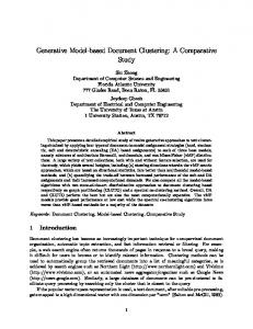
Figure 1.1: Individual category probabilities for the POM with five response categories Figure 1.1 shows a graphical representation of the POM for five response categories and one continuous predictor. As it can be seen, P (Y = k) has the same shape for all the ordinal categories (k = 2, . . . , q − 1) and differs only in its location. Alternatively, the POM has also a latent variable representation (Anderson & Philips 1981). Assuming that the ordinal response Y comes from


5

an underlying continuous response Y ∗ which follows a standard logistic distribution conditional on x such that Y = k if µk−1 ≤ Y ∗ ≤ µk , then the POM holds for Y. In other words, the POM could also be represented as Y ∗ = β ′ x + ϵ where ϵ ∼ Logistic(0, π 2 /3). Figure 1.2 shows a graphical representation, the ordinal response Y (right Y-axis) falls in category k = 1, 2, 3, 4 when the unobserved continuous response Y ∗ falls in the k th interval of values. The slope of the regression line is β.

Figure 1.2: Latent variable representation of the POM, reprinted from Agresti (2013). Maximum Likelihood (ML) methods are often used to fit cumulative logit models. ML estimates of the model parameters are obtained using iterative methods that solve the likelihood equations for all the cumulative logits, e.g. q − 1 equations in the case of the POM described above. Walker & Duncan (1967), McCullagh (1980) proposed the Fisher scoring

6


algorithm, an iteratively reweighted least squares algorithm, for this task. A sufficiently large n guarantees a global maximum but a finite n does not. In the latter, the ML function may exhibit local maxima or not have one at all (McCullagh 1980). When the POM fits poorly or the proportional odds assumption is inadequate, Liu & Agresti (2005) proposed the following potential alternative strategies. (i) Trying a model with separate effects, βk instead of β. This model however places additional constraints in the set of parameters µ and β to make sure that the cumulative probabilities are non-decreasing; (ii) Trying different link functions, (iii) Adding interactions or in general additional terms to the linear predictor; (iv) Adding dispersion terms; (v) Allowing separate effects, like in (i), for some but not all predictors. This model, introduced by Peterson & Harrell (1990), is called the Partial Proportional Odds model (PPOM); (vi) Using a model for nominal responses, e.g. Baseline logit. We next focus on option (iii) as it the most relevant for the purposes of this proposal. For a complete treatment see Liu & Agresti (2005). There are several ways to include additional terms to the linear predictor when there is lack of proportional odds. Here we present the Trend Odds Model (TOM) by Capuano & Dawson (2012) that will be extented later to the clustering case. The TOM is a monotone constrained nonproportional odds models that uses a logit link for the cumulative probability and adds an extra parameter γ to the linear predictor. Setting an arbitrary scalar tk that varies by ordinal outcome (k), the TOM has the form

Logit[P (Y ≤ k|x)] = µk − (β + γtk )′ x

tk ≤ tk+1 ; k = 1, . . . , q − 1

where µk − µk−1 ≥ γ(tk − tk−1 )x, ∀x is an additional constraint required to make sure the cumulative probabilities are non-decreasing. Intrinsically, therefore the TOM is a constrained model where for a given value of the


7

predictor, the odds parameter increases or decreases in a monotonic manner (γtk with tk ≤ tk+1 ) across the ordinal outcomes (k). Figure 1.3 shows a graphical representation of the TOM for five response categories and one continuous predictor. In contrast to the POM, figure 1.1, the probabilities for the ordinal responses P (Y = k) differ not only in their location but also in shape. For instance, the probability that the response is equal to the second category P (Y = 2) is no longer symmetric. Similarly, the probabilities that the response is equal to the first (P (k = 1)) and last (P (k = 5)) categories are no longer mirror images of each other.

Figure 1.3: Individual category probabilities for the TOM with five response categories Capuano & Dawson (2012) showed that the TOM is related to logistic, normal and exponential underlying latent variables and belongs to the class of constraint non-proportional odds models by Peterson & Harrell

8


(1990).

Other multinomial models Alternative probability models to analyse ordinal data include: cumulative link models, continuation-ratio logit models and adjacent-categories logit model. An important related model is the Stereotype model by Anderson (1984). Nested between the adjacent-categories logit model with proportional odds and the general baseline-category logit model, it captures any potential lack of proportionality by introducing new parameters for each category. Fernández et al. (2016) extend the Stereotype model to perform model based cluster analysis, see section 1.4. We note that these models belong within the class of multivariate generalised linear models (Multivariate GLM) whenever the response has a distribution in the exponential family (McCullagh 1980, Thompson & Baker 1981, Fahrmeir & Tutz 2001).

1.3 Models for repeated ordinal data Repeated ordinal data arise when an ordinal response is recorded at various occasions for each subject or unit, such as in longitudinal studies. We next discuss three main approaches to analyse such data: marginal models, subject-specific models and transitional models (Diggle et al. 2002, Vermunt & Hagenaars 2004, Agresti 2013). Marginal models, also known as population-averaged models, capture the effect of the predictor averaged over all the observations. Assume for simplicity that all responses repeat the same number of times T and let Yit be an ordinal response with q categories for individual i in occasion t. The marginal model with cumulative logit link has the form

Logit[P (Yit ≤ k|xit )] = µk −β ′ xit

k = 1, . . . , q−1; i = 1, . . . , n; t = 1, . . . , T.

1.3. MODELS FOR REPEATED ORDINAL DATA

9

where xit = (xit1 , xit2 , . . . , xitm )′ contains the values of the m predictors for individual i at occasion t. Model fitting is mostly performed using a generalised estimating equations (GEE) approach. This approach is a quasi likelihood method that only specifies the marginal regression models, over individuals i as in the equation above, and a working correlation structure, a guess specified by the analyst, among the T responses. Lipsitz et al. (1994) and Toledano & Gatsonis (1996) presented cumulative logit and probit models for repeated ordinal responses. Marginal models focus on the marginal distribution of Y by averaging over individual responses and treat the joint dependence structure as nuisance. Given that our aim is to explicitly classify subjects into latent clusters, we will not be using population-averaged approach in this dissertation. In contrast to that, subject-specific models describe effects at the individual or unit level. They are known by many names in the literature: conditional models, mixed effects models, random-effects models, and multilevel models. They jointly model the distribution of the response and the individual effects. Random effects models belong to the class of generalised linear mixed models (GLMM) when the response has a distribution in the exponential family. Individual effects are assumed to follow a certain probability distribution and hence their name of random effects. In our case, we use the random effects to capture the dependence among repeated responses but they could more generally be used to capture subject heterogeneity, unobserved covariates and other forms of overdispersion. The cumulative logit with random effects by subject has the form Logit[P (Yit ≤ k|xit )] = µk − β ′ xit − ai where k = 1, . . . , q − 1; i = 1, . . . , N ; t = 1, . . . , T and ai ∼ N (0, σ 2 ). This is the simplest model and is also known as the random intercept model. It could be extended to other ordinal models using different link functions as well as continuation-ratio logit models. ML estimation of these mod-

10


els is based on the marginal likelihood that integrates out the random effects. For simple cases like a random intercept Gauss-Hermite quadrature is used. In general, multiple random effects are possible but fitting for more than two terms is challenging (Tutz & Hennevogl 1996, McCulloch et al. 2008) due to the fact that the dimensionality of the integrals that need to be solved numerically grows with the number of random effects. Higherdimensional integrals are approximated through Monte Carlo simulation or pseudo-likelihood methods such as adaptative quadrature (Naylor & Smith 1982, Skrondal & Rabe-Hesketh 2004) and sequential Gaussian quadrature (Heiss 2008, Bartolucci et al. 2014). Of note here is the remark made by Pinheiro & Bates (1995) that quadrature and adaptive quadrature are deterministic versions of Monte Carlo integration and importance sampling. Quadrature methods need the selection of an adequate number of integration points. This is, however, a non- straightforward task and it has to be done case by case depending on the data at hand. For instance, in fitting a mixture of latent autoregressive models, Bartolucci et al. (2014) started with 21 quadrature points for a given number of mixture components and then increased it by 10 until convergence of the estimated log-likelihood was achieved. This scheme lead them to use 51 and 61 quadrature points for mixtures with one to 4 components. Moreover, as in all Frequentist estimation, the above methods only provide point estimates for the model parameters and confidence intervals need to be estimated in a separate step, usually using the Fisher information matrix which also needs to be approximated. In contrast to that, Bayesian approaches provide an attractive way forward. From the outset, Bayesian estimation aims to simulate the posterior distribution of parameters conditional on the data and thus provides estimates of the model parameters and their related uncertainty. Secondly, although multiple random effects might be more complex and take longer to simulate, thanks to the theory of Markov chains we are sure that a well

1.3. MODELS FOR REPEATED ORDINAL DATA

11

constructed MCMC chain will be able to efficiently explore any target distribution in finite time. Of course, a Bayesian approach is not a silver bullet that could be used for free. Issues such as the selection of priors, assessment of the convergence of the MCMC chain, and the design of MCMC moves for efficient exploration of the target distribution are of uttermost importance when using a Bayesian approach. Thanks to the advances in the Bayesian literature in the last decades, see for example Johnson & Al¨ bert (1999), Robert & Casella (2005), Fruhwirth-Schnatter (2006), Gelman ¨ et al. (2014), Muller et al. (2015), we now have a standard set of tools to tackle these issues. This together with the increase of computational power make Bayesian approaches a natural choice in complex models like the above. Chapter 5 presents a finite mixture for repeated ordinal data with latent random effects that follow a random walk with cluster-specific variance, and estimates it within a Bayesian framework. Finally, transitional models include also past responses as predictors. That is, they model the ordinal response Yt conditional on past responses Yt−1 , Yt−2 , . . . and other explanatory variables xt . A very popular transitional model is the first-order Markov model in which Yt is assumed to depend only on Yt−1 and covariates of time t. For example, Kedem & Fokianos (2005) used a cumulative logit transitional model in the context of a longitudinal medical study. In our case, Chapter 6 presents a finite mixture for repeated ordinal data with transitional terms by latent cluster and occasion and estimates it within a Bayesian framework. As remarked by Liu & Agresti (2005), the use of any of these three approaches depends on the problem at hand. That is, an approach should be chosen according to whether interpretations are needed at the population level, subject-specific predictions are of relevance, or whether or not it is important to describe effects of explanatory variables conditional on past responses. Furthermore, estimated effects can have different magnitude depending on the approach taken. For example, in transitional models the interpretation and magnitude of the effect of the past responses on the or-


12

dinal response depends on how many previous observations are include in the model. Also the effects of the other explanatory variables diminish markedly (Agresti 2013). In addition to that, effects in a subject-specific model are larger in magnitude than those in a population-averaged model.

1.4 Model based clustering analysis for ordinal data Traditional cluster analysis approaches treat ordinal responses as continuous and reduce the dimensionality of the data by using the eigenvalues and matrix decomposition. Amongst others, hierarchical clustering (Kaufman & Rousseeuw 1990) , association analysis (Manly 2005), and partition optimization methods like k-means clustering (Lewis et al. 2003), follow this approach. Since these approaches are not based on likelihoods, statistical inference tools are not available and model selection criteria can not be used to evaluate and compare different models. Model based approaches, such as Kendall’s τb (Kendall 1945), GoodmanKruskal’s γ (Goodman & Kruskal 1954) and Somers’ d (Somers 1962); also exists. However, they use distance metrics and similarity measures and thus do not fully exploit the ordinal structure of the data. Their associated statistical tests rely on Monte Carlo methods, testing only the sample at hand and not more general hypothesis about the data generating process. Hastie et al. (2009) presents full details. Model based clustering using finite mixtures have been proposed by several authors (Everitt & Hand 1981, McLachlan & Peel 2000). See a recent literature review by Fernández et al. (2017). This approach poses probabilistic models using finite mixtures which are mostly fitted using the Expectation-Maximisation algorithm (EM) (Dempster et al. 1977) and focus on either continuous, discrete or nominal responses. A major advantage of this approach is the availability of likelihoods, for the probability

1.4. MODEL BASED CLUSTERING ANALYSIS FOR ORDINAL DATA13 models, and therefore access to various model selection criteria to evaluate and compare different models. Finite mixtures are also known as Latent Class (LC) models in the literature of Latent Variable models (Bartholomew et al. 2011, Wedel & DeSarbo 1995). Used firstly in sociology (Lazarsfeld 1950), LC have been widely used to cluster ordinal responses, as well as continuous and categorical data. Although slight differences could be argued, McLachlan & Peel (2000) for instance points out that mixture components in LC models often represent actual underlying classes that may have a meaningful physical representation, both denominations have been used interchangeably in the literature even in early applications, see for example Aitkin’s seminal paper (Aitkin et al. 1981). In addition to that, this literature makes also an interesting connection of finite mixtures with random effects models. Here mixtures are a way to estimate models with discrete random effects since the distribution of the random effects is assumed to be multinomial across the latent classes. They accordingly use the terms nonparametric random-effects and non-parametric maximum likelihood (NPML) for the model and its estimation approach (Wedel & DeSarbo 1994, Aitkin 1996, Aitkin & Alfo´ 1998, Vermunt & Van Dijk 2001, Alfo` et al. 2016). Also of note in the latent variable literature are Skrondal & Rabe-Hesketh (2004) and Vermunt & Magidson (2000) who implemented this approach and made them available in standard software, GLLAMM (Generalised Linear Latent Mixed Models) and Latent Gold, respectively. It is important to stress that most of this literature has focused on parameter estimation and not clustering nor classification, that is the assignment of subjects to the latent classes. On the other hand, the latent variable literature has also had an almost exclusive reliance on AIC and BIC for model comparison (Nylund et al. 2007) which might not be appropriate for finite mixtures as it tends to overestimate the number of latent clusters (McLachlan & Peel 2000). Simultaneous clustering of row and columns is called biclustering, block


14

clustering or two-mode clustering. Biclustering models for binary, count and categorical data have been proposed by Biernacki et al. (2000), Pledger (2000), Govaert & Nadif (2008), Arnold et al. (2010), Labiod & Nadif (2011), Pledger & Arnold (2014). More recently, Matechou et al. (2016) and Fernández et al. (2016) have extended these models to ordinal responses. The former used the proportional odds (McCullagh 1980) and the latter the Stereotype model (Anderson 1984) and enable them to handle row, column and biclustered data. The overall aim of this dissertation is to extent these finite mixture models to the case of repeated ordinal data using the proportional odds formulation. This is done in Chapters 5, 6 and 7.

1.5 Model based clustering for repeated ordinal data In analogy to the literature for longitudinal data, there are two main approaches for finite mixture-based clustering for repeated ordinal data: mixtures of random effects models and mixtures of transitional models which we denote here parameter dependent (chapter 5) data dependent (chapter 6) models. These names are however just conventions as both approaches in turn could be viewed as special cases of non-linear state space models for longitudinal data (Fahrmeir & Tutz 2001) and models that combined both approaches could also be meaningful and have been proposed in the literature (Bates & Neyman 1952, Heckman 1981a, Skrondal & Rabe-Hesketh 2014).

1.5.1 Parameter dependent models Parameter dependent models, introduce the repeated measures correlation by conditioning the response on latent random effects, that is a finite mixture of random effects models. This is useful for instance to estimate time-varying unobserved heterogeneity as a mixture of discrete distribu-

1.5. MODEL BASED CLUSTERING FOR REPEATED ORDINAL DATA15 tions or stochastic processes (Vermunt et al. 1999, Vermunt & Van Dijk 2001, Bartolucci & Farcomeni 2009, Bartolucci et al. 2014). These models rely on the local independence assumption, that is conditional on the cluster membership, the random effects and potential observed covariates, the subjects are assumed to be independent. Vermunt & Van Dijk (2001) formulated a latent class regression model with class-specific coefficients, that is a finite mixture of random-intercepts and random-coefficients model. Given the lack of assumptions about the distribution of the random effects, the authors also viewed this model as a non-parametric two-level model. They applied this latent class regression model to responses with densities in the exponential family, including ordinal responses (Vermunt & Hagenaars 2004). More recently, Bartolucci et al. (2014) presented a mixture of latent auto-regressive models for longitudinal binary, categorical and ordinal data that includes covariates as well as time-varying unobserved heterogeneity as a mixture of AR(1), autoregressive processes of order one, with different correlation coefficients but sharing the same variance. Frequentist estimation is performed using EM and Newtown-Raphson (NR) algorithms with sequential Gaussian quadrature to integrate out the mixture distribution of random effects. Model comparison is carried out using BIC and the S-index that takes into account the level of separation of the mixture components. They provide an application to self-reported health status for 7074 individuals over 8 years in the USA and taking into account the entropy based S-index argued for a model with three components, although a model with four components had the lowest BIC. Latent Markov (LM) models (Wiggins 1973, Vermunt et al. 1999, Bartolucci et al. 2012) are another class of models that could also be considered parameter dependent. They are a generalization of finite mixtures where the cluster memberships arises from a discrete-state Markov chain and thus varies over time among the states. LM models are also known as Hidden Markov (HM) and Markov switching models in the time se-

16


ries literature (MacDonald & Zucchini 1997, Cappé et al. 2005, Zucchini & MacDonald 2009). LM and HM models are more flexible than finite mixtures but also less parsimonious since additional parameters for the initial states and a transition matrix between states need to be estimated. Among the important contributions on this area, we highlight Bartolucci (2006) that provided a restricted likelihood ratio test (RLRT) to compare different configurations of the transition matrix for a given number of latent states, including whether or not the transition matrix is diagonal. They thus provided a test for the comparison of the LM and finite mixture formulations of models with the same number of latent states. Ordinal data has been analysed using LM models by Vermunt et al. (1999) and Bartolucci & Farcomeni (2009). Vermunt et al. (1999) incorporates categorical time-constant and time-varying covariates to the LM for a categorical response, although they used the model for ordinal data. Importantly, in their formulation predictors affect initial and transition probabilities of the latent variable and not directly the response. The latter is also the case for Bartolucci & Farcomeni (2009), who proposed a multivariate extension of the dynamic logit model for binary, categorical and ordinal data. These authors used marginal logits for each response and marginal log-odds for each pair of responses and also allowed for covariates, including lagged responses. Their proposal moreover allows for time varying unobserved heterogeneity which is modelled as a first-order homogeneous Markov chain with a discrete number of states. The model is estimated using the EM and backward-forward recursions from the HM literature (MacDonald & Zucchini 1997) and model comparison is carried out using AIC and BIC. A simulation study shows how these information criteria worked well for the proposed model with BIC providing better results. They presented an application to fertility and employment as binary variables for 1446 women over 7 years. Using the AIC and the RLRT , they selected a LM model with three states which was preferred over the

1.5. MODEL BASED CLUSTERING FOR REPEATED ORDINAL DATA17 corresponding finite mixture model. Interestingly, using the BIC rendered a different result as the model with the lowest overall BIC was a finite mixture mixture (and not a LM) with four components. Chapter 5 presents a finite mixture model with latent random effects that encompasses the models of Vermunt & Van Dijk (2001) and Bartolucci et al. (2014) within one general framework. In particular, we propose a model with latent random effects that follow a standard normal distribution and Gaussian random walk process both cluster-specific variance. Our choice of sticking with finite mixtures, and not LM or HM models, was guided mainly by parsimony but also the aim of having both ways of modelling the time-varying unobserved heterogeneity within the same encompassing model. In contrast to these authors, we fit the models using a Bayesian approach and note their benefits and limitations in contrast to the Frequentist solutions.

1.5.2 Data dependent models Data dependent models, introduce the repeated measures correlation by conditioning on a finite mixture of previous responses, that is by allowing the lagged response to have a different effect on each cluster. These models are also known as Markov transition or latent transition models and typically use time-homogeneous first-order Markov chains with states corresponding to the levels of the response(s). The latter is the key defining characteristic of this approach, which contrast with the LM/HM models where the Markov chain is defined over unobserved states. Markov transition models have been used for model based clustering of longitudinal ¨ data and time series (Frydman 2005, Pamminger et al. 2010, FruhwirthSchnatter et al. 2012, Cheon et al. 2014). In addition to the local independence assumption, models within this approach have to deal with the initial conditions problem (Heckman 1981b, Wooldridge 2005) due to their use of lagged responses as predictors. That

18


is, a joint model for the cluster membership and the response that occurred previous to the initial one also has to be specified. Recently, Skrondal & Rabe-Hesketh (2014) provide advice on the main approaches to tackle this issue. ¨ Pamminger et al. (2010) and Fruhwirth-Schnatter et al. (2012) present a mixture-of-experts Markov chain clustering, a model based clustering approach for categorical time series that uses a finite mixture of transitional terms and include covariates in the group membership probabilities. Known as ”mixture-of-experts” in the machine learning literature, this model allows the covariate effects to be cluster specific and to deal with the initial conditions problem by adding the initial response into the set of regressors. This conditioning of the cluster membership on the initial response is an approach known as simple solution to the initial conditions problem in Econometrics (Wooldridge 2005). Model estimation is performed using MCMC and model selection with several Frequentist and Bayesian information criteria that take into account the entropy of the classification estimates. The models are illustrated using wage and income mobility in Austria. In both case studies, they found evidence for four latent groups with markedly different transitions over time. On the other hand, Frydman (2005), Cheon et al. (2014) developed restricted versions of the Markov transition models. Cheon et al. (2014) presents a disease progression model where the number of mixture components is equal to the disease states and thus is fixed in advance. Frydman (2005) considers another constrained model where the transition matrices for the latent groups are functions of the first group. ¨ Similarly to Pamminger et al. (2010) and Fruhwirth-Schnatter et al. (2012), the model proposed in Chapter 6 is a latent transition model that induces transition matrices that are completely unconstrained for all clusters. In contrast to them, the model we propose includes cluster-occasion interactions and thus the resulting transition matrices are time-varying. Furthermore, we construct the MCMC chain to sample from the target

1.6. THESIS ROADMAP

19

distribution in a different manner, apply a different relabelling algorithm (Stephens 2000), and use the newly developed Widely Applicable Information Criterion (WAIC) (Watanabe 2009, 2010) for model comparison.

1.6

Thesis Roadmap

In the chapters to follow, this dissertation develops clustering models based on finite mixtures to attempt to fill some of these gaps. These probability models are based on likelihoods and thus provide a fuzzy clustering approach in which observations could come from any latent cluster with some probability. In particular, we have developed several finite mixture models for two-way data in longitudinal settings. To ease comparability, we start off by formulating models where the occasions are assumed to be independent, using mixtures based on the Proportional Odds and Trend Odds models in Chapters 3 and 4, respectively and fitting them using the EM algorithm. We then proceed to model the correlation explicitly with mixtures that include latent random effects in Chapter 5, and latent transitional terms in Chapter 6. These latter models are fitted using a Bayesian approach to take advantage of the flexibility of MCMC methods to estimate models with complex correlation structures. Furthermore, in Chapter 7 we use a Dirichlet Process prior to estimate the number of mixture components within a Bayesian Non-Parametric approach. Throughout the dissertation, we validate the models using simulated data and also real data from socio-economic surveys and metagenomics. In particular, we used self-reported health status in Australia (poor to excellent), life satisfaction in New Zealand (completely agree to completely disagree) and site agreement with a reference genome (equal, segregating and variant) of bacteria from baby stool samples. More details of the these datasets are given next in Chapter 2.

20


Chapter 2 Data 2.1

Life Satisfaction (NZAVS)

The New Zealand Attitudes and Values survey (NZAVS) is a longitudinal survey hosted by the School of Psychology of the University of Auckland. It aims to study social attitudes, personality and health outcomes of New Zealanders. It was started in 2009 led by Associate Prof. Chris Sibley and now includes many researchers from a diverse range of research areas. Results and publication of all NZAVS data are independent of any specific funding agency or government body. About to start its 7th year, the NZAVS is a postal survey planned to be a 20-year long study extending to 2029. The sample frame from this survey is drawn from the New Zealand Electoral Roll and started with 6,518 people in 2009. Since then it has had a average retention rate of around 80%. Including booster samples from 2011, its sample frame includes about 22,000 unique people. More technical information about the NZAVS could be found at www.psych.auckland.ac.nz/uoa/NZAVS In this thesis, we use waves 1 to 5, 2009-2013, of self-reported ”Life Satisfaction” (LS). Specifically, participants were asked the following:

21

CHAPTER 2. DATA

22

The statements below reflect different opinions and points of view. Please indicate how strongly you disagree or agree with each statement. Remember, the best answer is your own opinion. Strongly Disagree I am satisfied with my life

1

Strongly Agree 2

3

4

5

6

7

LS is therefore an ordinal variable with seven levels, ranging from 1 (Strongly disagree) to 7 (Strongly Agree). Given that we use all individuals with complete responses between 2009 and 2013, this dataset has 2564 rows (n), 5 columns (p) and 7 ordinal levels (q). Over this period, most respondents exhibited very high levels of LS. As it can be seen in Figure 2.1, the majority of answers were very close to the highest end of the scale (5 to 7). In addition to that, there seems to be little variation of LS over time. Category 6 for instance was consistently just above 40% within this period. Similarly, categories 5 and 7 were around 20%. The remainder of categories all exhibited very low percentages, lower than 10% in the case of category 4 and lower than 5% in the case of categories 1,2 and 3. More in detail, Table 2.1 shows the distribution of LS in 2009 and 2013 as well as the transitions between ordinal categories in this period. This table shows for instance that 54% of people that responded 7 (”Strongly Agree”) in 2009 also have the same response in 2013. In general, people with positive perception of their LS (”Agree” and ”Strongly Agree”) have diagonals that are higher than 50% which means that they tend to similar perceptions at the beginning and end of the study period.

2.1. LIFE SATISFACTION (NZAVS)

23

Figure 2.1: Distribution of Life Satisfaction (LS) over 2009-2013 in the NZAVS

(1) Strongly Disagree (2) Disagree (3) Somewhat Disagree (4) Neither (5) Somewhat Agree (6) Agree (7) Strongly Agree

2009 0.01 0.02 0.04 0.10 0.23 0.39 0.20

2013 0.19 0.11 0.02 0.02 0.01 0.00 0.00

0.25 0.07 0.17 0.04 0.01 0.00 0.00

(1) (2) Strongly Somewhat Disagree Disagree 0.01 0.02 0.03 0.27 0.20 0.16 0.04 0.01 0.01

0.25 0.15 0.24 0.25 0.12 0.03 0.03

0.06 0.18 0.21 0.30 0.37 0.17 0.06

(3) (4) (5) Disagree Somewhat Disagree Neither Agree 0.04 0.08 0.22

Table 2.1: 2009-2013 transitions (%): Life Satisfaction in NZ

0.03 0.17 0.15 0.18 0.39 0.60 0.36

0.19 0.04 0.02 0.05 0.06 0.18 0.54

(7) Strongly Agree Agree 0.43 0.20

(6)

24

CHAPTER 2. DATA

2.1. LIFE SATISFACTION (NZAVS)

25

26

CHAPTER 2. DATA

2.2 Health Satisfaction (HILDA) The Household, Income and Labour Dynamics in Australia (HILDA) survey is a household panel study which began in 2001 and collects information about economic and subjective well-being, labour market dynamics and family dynamics in Australia. The HILDA Project was initiated and is funded by the Australian Government Department of Social Services (DSS) and is managed by the Melbourne Institute of Applied Economic and Social Research (Melbourne Institute). Wave 1 in the panel had 7,682 households and 19,914 individuals and was topped up with an additional 2,153 households and 5,477 individuals in wave 11. More information about this survey can be found at: www.melbourneinstitute.com/hilda/ We use self-reported health status (SRHS) in 2001-2011 from this dataset. Using a five-level scale (Poor, Fair, Good, Very Good and Excellent) each year respondents answer the following question: ”In general, would you say your health is:”. We use individuals with complete records over 2001 to 2011, or 11 occasions. Therefore, for the HILDA dataset we have n = 4660 rows , p = 11 columns and q = 5 ordinal levels. Figure 2.2 shows the distribution of SRHS in 2001 and 2011. In 2001, most individuals reported ”Very Good” and ”Good” health. About an eighth reported their health as ”Excellent” and about a tenth as ”Fair”. A very low number of individuals said their health was ”Poor”. In contrast to that, in 2011 the same individuals reported lower health levels. ”Excellent” and ”Very Good” answers decreased and ”Poor” and ”Fair” increased. Overall, SRHS’s distribution slightly shifted to the left and is thus more symmetric in 2011 than in 2001. Furthermore, for each individual SRHS is highly correlated across time. Table 2.2 presents the 2001-2011 transitions between ordinal categories for all individuals. Diagonal proportions are very high, about 40%, and the same is true for the cells close to the diagonal. In words, even after 11 years individuals are very likely to report a very similar health status. The

2.2. HEALTH SATISFACTION (HILDA)

27

only exception to this, is people that responded ”Excellent” in 2001. They have a slighter less positive perception of their health as 47% moved to ”Very Good” over this period. Table 2.2: SRHS transition matrix 2001-2011

Poor Fair 2001 Good Very Good Excellent

Poor

Fair

0.42 0.13 0.02 0.01 0.01

0.40 0.44 0.21 0.09 0.04

2011 Good Very Good Excellent 0.14 0.34 0.54 0.38 0.21

0.04 0.07 0.20 0.46 0.47

0.00 0.01 0.02 0.07 0.27

Total 1.00 1.00 1.00 1.00 1.00

CHAPTER 2. DATA

28

2001

2011 Figure 2.2: Distribution of Self-Reported Health Status (SRHS) in 2001 and 2011 in HILDA

2.3. INFANT GUT BACTERIA (METAGENOMICS)

2.3

29

Infant gut bacteria (Metagenomics)

Metagenomics uses samples found in the physical environment to study genetic material. This contrasts with many other areas of Genomics where cultured samples are used. This dataset is a timeseries of infant gut bacterial composition that allows us to observe the developing of the infant gut. The main inferential goal when using this kind of data is to shed light on the dynamics of the (latent) strains of bacteria (b.faecis) that compete to inhabit the human gut after birth. Figure 2.3 shows the sampling timeline.

Figure 2.3: Infat gut sampling timeline. Source: Chan et al. (2015) More in detail, this dataset consists of reference and variant allele counts for 62,996 single-nucleotide variant (SNV) sites, specific positions in the genome of the bacteria, followed over 45 days. These counts are then used to produce and ordinal variable, infant gut bacteria variants, with three levels:”fixed to reference”, ”segregating site”, and ”fixed to a nonreference”. At each time point, these levels are defined as follows • ”fixed to reference”: includes SNV sites where all reads are the same as the reference; • ”segregating site” more than 5 reads are equal to reference and more

CHAPTER 2. DATA

30 than 5 reads are equal to a different one;

• ”fixed to non-reference” all reads for the cell are the same allele which is different to the reference one. Figure 2.4 shows a heatmap of the data using yellow, red and blue for these levels. Fitting a Poisson mixture for the reads with Automatic Differentiation Variational Inference, Chan et al. (2015) found evidence for at least three strains, that is at least three different patterns of reads overtime. Given the large size of this dataset and the amount of missing observations, sites with no reads at all, we use all observations with complete data over the first 25 occasions. Thus, the infant gut dataset has n = 1992 rows, p = 25 columns and q = 3 ordinal levels and is publicly available at my personal repository: bitbucket.org/cholokiwi/nzsa2016/src.

2.3. INFANT GUT BACTERIA (METAGENOMICS)

31

Figure 2.4: Heatmap for infant gut bacteria variants over 45 days. Source: Chan et al. (2015)

32

CHAPTER 2. DATA

Part I Frequentist Estimation

33

Chapter 3 Proportional Odds Model 3.1

The Model

In this chapter, we extend the Proportional Odds Model (POM) by McCullagh (1980) to the case of latent groups. That is, we introduce unobserved covariates into the linear predictor of the cumulative probability of observing the ordinal outcomes. We already introduced this model in the previous chapter (Section 1.2). As a starting point, the models in this chapter assume that the observations are independent over time. By doing so, we thus use the same framework as Matechou et al. (2016). The setup that follows will be used throughout the present as well as in Chapters 3, 4, 5 and 6. Let data Y be a (n, p) matrix where each cell yij is equal to any of the q ordinal categories, where: i = 1, ..., n ; j = 1, ..., p and k = 1, ..., q. This is, each response yij is the realization of a multinomial ∑ distribution with probabilities θij1 , . . . θijq , where θijk ≥ 0 and qk=1 θijk = 1. We also define an indicator variable I(yij = k) equal to 1 if the condition yij = k is satisfied and 0 otherwise. v represents the number of model parameters. 35

CHAPTER 3. PROPORTIONAL ODDS MODEL

36 Saturated model

We begin by formulating a model where every single row (i) and column (j) and its interactions have an effect in the linear predictor of the POM, the saturated model Logit[P (yij ≤ k)] = µk − αi − βj − γij

(3.1)

where i = 1 . . . n, j = 1 . . . p, k = 1, . . . , q and the following identifiability constraints: α1 = 0 β1 = 0 γ1j = 0, ∀j; γi1 = 0, ∀i µk−1 < µk , k = 1, . . . , (q − 1) and µ0 = −∞, µq = ∞ The parameter µk is the k th cut point, αi is the effect of row i, βj is the effect of column j and γij is an interaction effect between row i and column j. The model can also be expressed in terms of the probabilities of each ordinal outcome θijk

P (yij = k) = θijk =

1 1+

e−(µk −αi −βj −γij )

−

1 1+

e−(µk−1 −αi −βj −γij )

This model is not at all parsimonious as it has v = (q − 1) + (n − 1) + (p − 1) + (n − 1)(p − 1) parameters. Row and column effects model A more parsimonious alternative is the model with only main row (i) and column (j) effects Logit[P (yij ≤ k)] = µk − αi − βj or

(3.2)

3.1. THE MODEL

37

1

P (yij = k) = θijk =

e−(µk −αi −βj )

1

−

e−(µk−1 −αi −βj )

1+ 1+ This model has the same constraints on µ, α, β as above and it has v = (q −1)+(n−1)+(p−1) parameters. v is still potentially large and increases linearly with the sample size. More parsimonious alternatives are thus needed. Row-clustering only Suppose now that each row belongs to one of the r = 1, . . . , R row groups with probabilities π1 , . . . , πR . That is, we assume that the rows come from a finite mixture with R components where both R and the group member∑ ship ri are unknown. Note that R < n and πr ≥ 0, R r=1 πr = 1, ∀i. Now, let θrjk be the probability that observation yij equals ordinal category k given that row i belongs to row-cluster r: P (yij = k|i ∈ r) = θrjk . In this simple case, row-clustering only with no column effects, the model is: Logit[P (yij ≤ k|i ∈ r)] = µk − αr

(3.3)

which implies θrjk =

1 e−(µk −αr )

−

1 e−(µk−1 −αr )

1+ 1+ Here α1 = 0, and µk−1 < µk , k = 1 . . . (q − 1), µ0 = −∞ and µq = ∞. µk is the k th cut-off point and αr is the effect of row-cluster r. Assuming independence over the rows and, conditional on the rows, independence over the columns, the likelihood becomes L(ϕ, π|Y ) =

n ∑ R ∏ i=1 r=1

πr

p q ∏ ∏

I(y =k)

θrjkij

(3.4)

j=1 k=1

where ϕ = (µ, α) is the set of parameters in the linear predictor. The expression above is also referred as the incomplete data likelihood given that


38

the cluster memberships of the rows are unknown. The number of model parameters is equal to: v = (q − 1) + 2(R − 1). Note that the linear predictor in this simple case does not depend on the columns (j) and thus we could have also written θrjk as θrk . Row-clustering with column effects To introduce column effects we augment the linear predictor to Logit[P (yij ≤ k|i ∈ r)] = µk − αr − βj

(3.5)

which implies P (yij = k|i ∈ r) = θrjk =

1 1+

e−(µk −αr −βj )

1

−

1+

e−(µk−1 −αr −βj )

(3.6)

where α1 = β1 = 0, and µk−1 < µk , k = 1 . . . (q − 1). µk is the k th cut-off point, αr is the effect of row-cluster r and βj the effect of column j. In this case, the likelihood is L(ϕ, π|Y ) =

n ∑ R ∏ i=1 r=1

πr

p q ∏ ∏

I(y =k)

θrjkij

(3.7)

j=1 k=1

where: ϕ=(µ, α, β) and the number of parameters in the model is v = (q − 1) + 2(R − 1) + (p − 1). Row-clustering with column effects and interactions To introduce column effects and interactions in the row-clustered model, we further augment the linear predictor to Logit[P (yij ≤ k|i ∈ r)] = µk − αr − βj − γrj

(3.8)

which is equivalent to P (yij = k|i ∈ r) = θrjk =

1 1+

e−(µk −αr −βj −γrj )

−

1 1+

e−(µk−1 −αr −βj −γrj )

3.1. THE MODEL

39

Where α1 = β1 = 0; γ1j = 0, ∀j; γr1 = 0, ∀r; and µk > µk−1 , k = 1 . . . (q − 1). µk is the k th cut-off point, αr is the effect of row-cluster r, βj the effect of column j and γrj the row-cluster and column interaction. The likelihood for this model is p q n ∑ R ∏ ∏ ∏ I(y =k) L(ϕ, π|Y ) = (3.9) πr θrjkij i=1 r=1

j=1 k=1

where: ϕ = (µ, α, β, γ) and the number of model parameters v = (q − 1) + 2(R − 1) + (p − 1) + (R − 1)(p − 1). Column-clustering only Column-clustering is also one-way clustering and is equivalent to rowclustering with the transposed data. That is, we could obtain column groups by exchanging row and columns and applying the row-cluster model from the previous section. Setting C as the number of mixture components, κc as the mixture proportion for group c, and P (yij = k|j ∈ c) = θick , the model becomes Logit[P (yij ≤ k|j ∈ c)] = µk − βc

(3.10)

or alternatively P (yij = k|j ∈ c) = θick =

1 e−(µk −βc )

−

1 e−(µk−1 −βc )

1+ 1+ where β1 = 0, and µk−1 < µk , k = 1 . . . (q − 1). µk is the k th cut-off point and βc is the effect of column-cluster c. Note also that C < p and ∑ κc ≥ 0, C c=1 κc = 1. Assuming independence over the columns and independence over the rows conditional on the columns, the model’s likelihood is L(ϕ, κ|Y ) =

p C ∏ ∑ j=1 c=1

κc

q n ∏ ∏

I(y =k)

θick ij

(3.11)

i=1 k=1

where ϕ = (µ, β). The incomplete information likelihood for this only column-cluster case has v = (q − 1) + 2(C − 1) parameters.


40

Column-clustering with row-effects We introduce row-effects to the column-clustering by augmenting the model in (3.10) to Logit[P (yij ≤ k|j ∈ c)] = µk − βc − αi

(3.12)


1 1+

e−(µk −βc −αi )

−

1 1+

e−(µk−1 −βc −αi )

where β1 = α1 = 0, and µk−1 < µk , k = 1 . . . (q − 1). µk is the k th cut-off point, βc is the effect of column-cluster c and αi the effect of row i. Note ∑ also that C < p and C c=1 κc = 1. Its likelihood is then L(ϕ, κ|Y ) =

p C ∏ ∑

κc

j=1 c=1

q n ∏ ∏

I(y =k)

θick ij

(3.13)

i=1 k=1

where ϕ = (µ, β, α) and v = (q − 1) + 2(C − 1) + (n − 1) parameters. Column-clustering with row-effects and interactions In this case, the model is described by Logit[P (yij ≤ k|j ∈ c)] = µk − βc − αi − γic

(3.14)


1 1 + e−(µk −βc −αi −γic )

−

1 1 + e−(µk−1 −βc −αi −γic )

here β1 = α1 = 0; γi1 = 0, ∀i; γ1c = 0, ∀c; and µk−1 < µk , k = 1 . . . (q − 1). µk is the k th cut-off point, βc is the effect of column-cluster c, αi the effect of row i and γic the column-cluster and row interaction. The likelihood for this model is L(ϕ, κ|Y ) =

p C ∏ ∑ j=1 c=1

κc

q n ∏ ∏ i=1 k=1

I(y =k)

θick ij

(3.15)

3.1. THE MODEL

41

with ϕ = (µ, β, α, γ) and v = (q − 1) + 2(C − 1) + (n − 1) + (C − 1)(n − 1) parameters. Bi-clustering Bi-clustering is also known as two-way, two-mode and latent block clustering (Govaert & Nadif 2010, Pledger & Arnold 2014, Matechou et al. 2016) and it consists of simultaneous clustering of the rows and columns. Here, it is assumed that rows come from a finite mixture with R row groups while the columns come from a finite mixture with C column groups, simultaneously. The row and column-cluster proportions are π1 , . . . , πR and κ1 , . . . , κC , respectively. R, C, πr and κc are unknown. Note that R < n, ∑C ∑ C < p, R c=1 κc = 1. r=1 πr = 1 and Let θrck = P (yij = k|i ∈ r ∩j ∈ c) be probability that cell (i, j) is equal to ordinal outcome k given that it belongs to row group r and column group c. Keeping as before αr and βc , for the row and column-cluster effects, the linear predictor becomes: Logit[P (yij ≤ k|i ∈ r ∩ j ∈ c)] = µk − αr − βc

(3.16)

or alternatively

P (yij = k|i ∈ r ∩ j ∈ c) = θrck =

1 1+

e−(µk −αr −βc )

−

1 1+

e−(µk−1 −αr −βc )

Where α1 = β1 = 0 and µk−1 > µk , k = 1 . . . (q − 1), µ0 = −∞ and µq = ∞. In this case, the likelihood sums over all possible partitions of rows into R clusters and over all possible partitions of columns into C clusters. Assuming independence over the rows and independence over the columns conditional on the rows, the incomplete data likelihood could be simplified to L(ϕ, π, κ|Y ) =

C ∑ c1 =1

···

C ∑ cp =1

κc1 . . . κcp

n ∑ R ∏ i=1 r=1

πr

p q ∏ ∏ j=1 k=1

I(y =k)

θrcj kij

(3.17)


42

where ϕ = (µ, α, β). This expression is computationally expensive to evaluate since it requires consideration of all possible allocations of the p columns to the C groups. Alternatively, assuming independence over the columns and independence over the rows conditional on the columns, it simplifies to L(ϕ, π, κ|Y ) =

R ∑

···

r1 =1

R ∑

πr1 . . . πrn

rn =1

p C ∏ ∑ j=1 c=1

κc

q n ∏ ∏

I(y =k)

θri ckij

(3.18)

i=1 k=1

Likewise (3.17), ( 3.18) is very expensive to compute due to requiring consideration of all possible allocations of the n rows to the R groups. In either specification, the incomplete data likelihood for the bi-clustering has v = (q − 1) + 3(R + C − 2) parameters.

Bi-clustering with interactions In this case, the model is Logit[P (yij ≤ k|i ∈ r ∩ j ∈ c)] = µk − αr − βc − γrc

(3.19)

or alternatively P (yij = k|i ∈ r ∩ j ∈ c) = θrck =

1 1+

e−(µk −αr −βc −γrc )

−

1 1+

e−(µk−1 −αr −βc −γrc )

Where α1 = β1 = 0; γ1c = 0, ∀c; γr1 = 0, ∀r; and µk > µk−1 , k = 1 . . . (q − 1), µ0 = −∞ and µq = ∞. µk is the k th cut-off point, αr is the r row-cluster effect, βc is the c column-cluster effect and γrc the row-cluster and column-cluster interaction. Depending on the independence assumptions, over the rows conditional on the columns or vice versa, the likelihood for this model is the same as in (3.17) or (3.18) with the augmented linear predictor ϕ = (µ, α, β, γ).

3.2. FREQUENTIST ESTIMATION

3.2

43

Frequentist Estimation

In this section we use a Frequentist framework to maximise the likelihoods described above and estimate the model parameters. In particular we use the Expectation-Maximization (EM) algorithm (Dempster et al. 1977). In essence, the EM algorithm turns the estimation into a missing data problem and then estimates the parameters using an iterative two-fold approach. In the case of finite mixtures, it first introduces new variables for the unknown group memberships. It then initialises these missing data given some initial values for the parameters (E-step). Secondly, the parameters are estimated by maximizing the likelihood given the estimated missing data (M-step). This likelihood is known as ”complete data” likelihood since is assumes that the latent group memberships are known. The new parameters in turn are fed to the E-step again and the process repeats until the parameters converge, that is when the change in the parameters and/or the likelihood is tiny. Row-clustering Let zir be the latent row group memberships for each row. zir is an indicator function equal to 1 if row i belongs to cluster r and 0 otherwise. It is not ∑ observed and thus is regarded as missing data. Note that R r=1 zir = 1, ∀i, and we define a membership matrix Z(n,R) to gather together all the zir ’s. As before ϕ denotes the linear predictor parameters so that the parameters of the model are (ϕ, π). Given a value for the number of mixture components R, the EM algorithm proceeds as follows. E-step: Estimate Z. Given Y and initial values for ϕ and π, estimate the expected value of zir as E[zir |Y, ϕ, π] =ˆ zir =

∏p

∏q

I(yij =k) k=1 θrjk ∑R ∏p ∏q I(yij =k) π a a=1 j=1 k=1 θajk

πr

j=1

(3.20)


44

In words, zîr is the posterior probability that observation yij belongs to ∑ the (row) mixture component r. R îr = 1, ∀i. r=1 z M-step: Numerically maximise the complete data log-likelihood. Given zîr from the E-step maximise ℓc to obtain new values for ϕ and π

ℓc (ϕ, π|Y, Z) =

p q R ∑ n ∑ ∑ ∑ i=1 j=1 r=1 k=1

zîr I(yij = k) log(θrjk ) +

n ∑ R ∑

zîr log(ˆ πr )

i=1 r=1

(3.21) îr /n. That is, the mixing proportions πˆr are i=1 z

∑n

where π ˆr = E[πr |Z] = first obtained using Z. A new cycle starts when the parameters from the M-step are used in the E-step and the Z matrix is re-estimated. This process repeats until estimates for ϕ have converged. The parameters in the linear predictor depend on type of clustering we are performing. For the row-clustering case we have ϕ = (µ, α), for rowclustering with column effects ϕ = (µ, α, β) and for row-clustering with column effects and interactions ϕ = (µ, α, β, γ). Importantly, as with any other maximization algorithm, there is a risk of convergence to local maxima due to multimodality of the likelihood. It is thus important to start the EM algorithm with several widely spread initial values, McLachlan & Peel (2000), and check that all of them converge to the same place. (log-likelihood value) Column-clustering Let xjc be the latent column-cluster memberships for each column j and ∑ X the membership matrix where each cell is equal to xjc , C c=1 xjc = 1. Given a value for the number of mixture components C, the EM algorithm proceeds as follows. E-step: Estimate X. Given Y and initial values for ϕ, we estimate the expected values of xjc as

3.2. FREQUENTIST ESTIMATION

E[xjc |Y, ϕ, κ] = xˆjc =

45 ∏n ∏q

I(yij =k) k=1 θick ∑C ∏n ∏q I(yij =k) a=1 κa i=1 k=1 θiak

κc

i=1

(3.22)

That is, xˆjc is the posterior probability that observation yij belongs to the (column) mixture component c. M-step: Numerically maximise the complete data log-likelihood. Given xîr from the E-step maximise ℓc to obtain new values for ϕ and κ

ℓc (ϕ, κ|Y, X) =

p q n ∑ C ∑ ∑ ∑ i=1 j=1 c=1 k=1

where κ ˆ c = E[κc |X] = first obtained using X.

∑p j=1

xˆjc I(yij = k) log(θick ) +

p C ∑ ∑

xˆjc log(ˆ κc )

j=1 c=1

(3.23) xˆjc /p. That is, the mixing proportions κˆc are

A new cycle starts when the parameters from the M-step are use in the E-step. This process repeats until convergence for ϕ. Again, the parameters in the linear predictor depend on type of clustering used: ϕ = (µ, α), ϕ = (µ, α, β), and ϕ = (µ, α, β, γ) for the column-clustering, columnclustering with row effects, and column-clustering with row effects and interactions, respectively. Bi-clustering Let zir and xjc be the latent row and column cluster memberships for each cell (i, j). As before Z and X are membership matrices formed by all the ∑C ∑ zir , xjc values. Note that R c=1 xjc = 1. Let ϕ be the set of model r=1 xir = parameters for the biclustering case, we also incorporate the variational approximation employed by Govaert & Nadif (2005) E[zir xjc |Y, ϕ] ≃ E[zir |Y, ϕ]E[xjc |Y, ϕ] = zîr xˆjc That is, conditonal on the ordinal response and the parameters the effect of the row and column clusters are independent. Given this approxi-


46

mation, values for the number of mixture components (R, C), and assuming independence over the rows and independence over the columns conditional on the rows, the EM algorithm proceeds as follows. E-step: Estimate Z and X. Given Y and initial values for ϕ estimate the expected values of zir and xjc as

πr E[zir |Y, ϕ, π] = zîr = ∑ R

∏p j=1

{∑ C

c=1 κc {∑ C

∏q

I(yij =k) k=1 θrck

}

} ∏p ∏q I(yij =k) π κ θ a b a=1 j=1 b=1 k=1 abk } ∏n {∑R ∏q I(yij =k) κc i=1 π θ r=1 r k=1 rck } {∑ E[xjc |Y, ϕ, κ] = xˆjc = ∑ ∏q ∏ I(yij =k) R n C k=1 θabk a=1 πa i=1 b=1 κb

(3.24)

M-step: Numerically maximise the complete data log-likelihood. Given zîr and xˆjc from the E-step maximise ℓc to obtain new values for ϕ, π, κ

ℓc (ϕ, π, κ|Y, Z, X) =

q p n ∑ R ∑ C ∑ ∑ ∑

zîr xˆjc I(yij = k) log(θrck )

i=1 j=1 r=1 c=1 k=1

+

+

n ∑ R ∑ i=1 r=1 p C ∑ ∑

(3.25)

zîr log(ˆ πr ) xˆjc log(ˆ κc )

j=1 c=1

where: πˆr = E[πr |Z] =

∑n

îr /n and κˆc = E[κc |X] = i=1 z

∑p j=1

xˆjc /p.

A new cycle starts when the parameters from the M-step are use in the E-step. This process repeats until convergence. Note that θrck is estimated using the corresponding linear predictor, bi-clustering in (3.16) and bi-clustering with interactions in (3.19).

3.3. SIMULATIONS

3.3

47

Simulations

In this chapter, we use synthetic datasets to illustrate the performance of the models presented so far. In particular, we simulate several scenarios and evaluate the performance of the POM model with row-clustering and column effects ( 3.5). This model is more complex than the POM model with row-clustering but more parsimonious than the POM model with row-clustering with column effects and interactions. We generate a total of 18 scenarios with varying sample size (3), number of columns (2) and mixture proportions (3). We use the following setup: • R = 3 number of mixture components • µ = (−2.08, −1.39, 1.39, 2.08) cut points • q = 5 ordinal levels, • α = (0, −2, 3) cluster effects • β = (0, 0.15, 0.30, . . . , 0.15(p − 1)) column effects. Given this setup, the model has v = 12 and 17 parameters, for p = 5 and 10, respectively. Table 3.1 details these scenarios Table 3.1: Labels for the scenarios (1-18) in the simulation study

π = (0.50, 0.30, 0.20) π = (0.33, 0.33, 0.34) π = (0.90, 0.08, 0.02)

60

p=5 n 200 1000

p = 10 n 60 200 1000

1 7 13

2 8 14

4 10 16

3 9 15

5 11 17

6 12 18

For each scenario, we generate 500 simulated datasets with 20 random initial values each to avoid the risk of convergence to local maxima. We

48


therefore estimate 3 × 2 × 3 × 500 × 20 = 180, 000 models overall. We estimate the model parameters using the EM algorithm as detailed in Section 3.2. Convergence is set to a maximum change of 10−8 in the absolute value of all the parameter estimates between EM iterations. The models are implemented in R (R 3.2.2) and C++. In particular, estimation in the Mstep is carried out using the optim() function in R and the corresponding log-likelihoods in C++ compiled functions. Tables 3.2 to 3.8 and figures 3.1 to 3.4 present the results. We start with scenarios 1-6 in Tables 3.2 and 3.3 where the mixture proportions π = (0.20, 0.30, 0.50) are unbalanced but the smallest component is not too small. Overall, we could see that the means of estimated parameters are close to their true values for all the model parameters. That is, the estimates for the cut-off points µ, cluster effects α, column effects β, and mixture proportions π all seem to converge to their true values. The standard deviations of these estimates are large for the n = 60 sample size. This is not surprising since we are estimating v = 12 independent parameters with only 60 rows and 5 columns. Increasing n has the effect of both providing estimates closer to their true values and decreasing the standard errors. For n = 1000 the mean values are already very close the true ones with small standard errors. Scenarios 4-6 present the estimates with twice the number of columns (p = 10 instead of p = 5). The model in this case has v = 17 independent parameters. Table 3.3 shows that the mean values of the estimates are close to the true parameter values with decreasing standard deviations in n. Furthermore, these estimates exhibit lower variability than the previous ones. Looking closely into the estimates of cluster effects αr , Figure 3.1 presents all the estimates for α over the 500 replicated datasets. It is evident that bigger n provides closer estimates to the true value for α. However, there seem to be some estimates that are very different from the true values. For example for n = 60 and p = 5 there are estimates near the axis and thus are clearly far off from the true values (−2, 3) in the middle of the graph.

3.3. SIMULATIONS

49

Importantly, these outliers disappear when n or p increase. Table 3.2: Scenarios 1-3. Estimated parameters for the POM with rowclustering and column effects. Mean and standard deviation (sd) over 500 simulated datasets. π = (0.50, 0.30, 0.20) and p = 5.

Param

true

n = 60 mean sd

n = 200 mean sd

n = 1000 mean sd

µ1 µ2 µ3 µ4

-2.08 -1.39 1.39 2.08

-2.21 -1.49 1.34 2.05

0.58 0.58 0.58 0.60

-2.10 -1.40 1.40 2.11

0.24 0.23 0.21 0.22

-2.08 -1.39 1.39 2.09

0.10 0.10 0.09 0.10

α1 α2 α3

0.00 -2.00 3.00

0.00 -2.16 3.04

0.00 0.40 0.65

0.00 -2.05 3.05

0.00 0.19 0.24

0.00 -2.00 3.01

0.00 0.09 0.11

β1 β2 β3 β4 β5

0.00 0.15 0.30 0.45 0.60

0.00 0.18 0.30 0.48 0.64

0.00 0.38 0.39 0.37 0.39

0.00 0.15 0.30 0.46 0.61

0.00 0.20 0.22 0.20 0.20

0.00 0.15 0.30 0.45 0.60

0.00 0.09 0.09 0.09 0.09

π1 π2 π3

0.50 0.30 0.20

0.48 0.32 0.20

0.12 0.13 0.06

0.50 0.30 0.20

0.06 0.06 0.03

0.50 0.30 0.20

0.03 0.03 0.01


50

Table 3.3: Scenarios 4-6. Estimated parameters for the POM with rowclustering and column effects. Mean and standard deviation (sd) over 500 simulated datasets. π = (0.50, 0.30, 0.20) and p = 10.

Param

true

n = 60 mean sd

n = 200 mean sd

n = 1000 mean sd

µ1 µ2 µ3 µ4

-2.08 -1.39 1.39 2.08

-2.12 -1.42 1.40 2.10

0.33 0.31 0.29 0.30

-2.09 -1.39 1.40 2.10

0.18 0.17 0.16 0.17

-2.08 -1.39 1.39 2.08

0.07 0.07 0.07 0.07

α1 α2 α3

0.00 -2.00 3.00

0.00 -2.04 3.05

0.00 0.22 0.31

0.00 -2.01 3.03

0.00 0.11 0.16

0.00 -2.00 3.00

0.00 0.05 0.07

β1 β2 β3 β4 β5 β6 β7 β8 β9 β10

0.00 0.15 0.30 0.45 0.60 0.75 0.90 1.05 1.20 1.35

0.00 0.17 0.28 0.46 0.63 0.76 0.91 1.06 1.20 1.37

0.00 0.35 0.36 0.37 0.38 0.38 0.36 0.37 0.37 0.36

0.00 0.16 0.30 0.45 0.60 0.76 0.92 1.06 1.22 1.35

0.00 0.21 0.20 0.20 0.19 0.21 0.21 0.20 0.20 0.21

0.00 0.15 0.30 0.45 0.59 0.74 0.90 1.05 1.20 1.35

0.00 0.09 0.09 0.09 0.09 0.09 0.09 0.09 0.09 0.09

π1 π2 π3

0.50 0.30 0.20

0.50 0.31 0.20

0.08 0.07 0.05

0.50 0.30 0.20

0.04 0.04 0.03

0.50 0.30 0.20

0.02 0.02 0.01

3.3. SIMULATIONS

51

Tables 3.4 and 3.5 present the results for scenarios 7-12, which have balanced mixture proportions π = (0.33, 0.33, 0.34). In general, the means of estimated parameters are also close to their true values for all the model parameters. However, the main difference of these new scenarios is that the variability of these estimates (sd) is very similar among all the mixture components. This is somewhat expected as all the mixture components are equally represented in the data. On the other hand, occasional outliers seem to be also present in the estimates of the cluster effects α, Figure 3.2, but they dissapear as n and p grow. Table 3.4: Scenarios 7-9. Estimated parameters for the POM with rowclustering and column effects. Mean and standard deviation (sd) over 500 simulated datasets. π = (0.33, 0.33, 0.34) and p = 5.

Param

true

n = 60 mean sd

µ1 µ2 µ3 µ4 α1 α2 α3 β1 β2 β3 β4 β5 π1 π2 π3

-2.08 -1.39 1.39 2.08 0.00 -2.00 3.00 0.00 0.15 0.30 0.45 0.60 0.33 0.33 0.34

-2.36 -1.65 1.18 1.91 0.00 -2.31 3.01 0.00 0.21 0.33 0.48 0.66 0.32 0.36 0.32

0.75 0.76 0.77 0.77 0.00 0.77 0.74 0.00 0.36 0.36 0.37 0.38 0.11 0.13 0.08

n = 200 mean sd

n = 1000 mean sd

-2.11 -1.41 1.38 2.07 0.00 -2.05 3.02 0.00 0.15 0.30 0.45 0.62 0.33 0.33 0.34

-2.08 -1.39 1.39 2.08 0.00 -2.00 3.00 0.00 0.15 0.30 0.45 0.60 0.33 0.33 0.34

0.30 0.30 0.27 0.28 0.00 0.22 0.24 0.00 0.21 0.22 0.21 0.21 0.05 0.06 0.04

0.13 0.13 0.12 0.12 0.00 0.09 0.10 0.00 0.09 0.09 0.08 0.09 0.02 0.02 0.02


52 ●

●

n= 60 ●

n= 60

2.0

●

4.5 4.0 3.5 2.5

●

●

1.5

1.5

● ● ●

−3.5

−3.0

−2.5

−2.0

−1.5

−1.0

−0.5

−3.5

−2.0

α2

n= 200

n= 200

−1.5

−1.0

−0.5

−1.0

−0.5

−1.0

−0.5

4.5 4.0 3.5 2.0 1.5

1.5

2.0

2.5

α3

●●● ● ●●● ● ● ● ●●● ● ● ● ● ● ● ● ● ● ● ● ● ● ●● ●● ● ●●● ● ●●● ● ● ● ● ● ● ● ● ● ●●● ● ● ● ● ● ● ● ● ● ● ● ● ● ● ● ● ● ● ● ● ● ● ● ● ● ● ●● ● ● ● ● ● ● ● ● ● ● ● ● ● ● ● ● ● ● ● ●● ● ● ● ● ● ● ●● ● ● ● ● ● ● ● ● ● ● ● ● ● ● ● ● ● ●● ● ● ● ● ● ● ● ● ● ● ● ● ● ● ● ● ● ● ● ● ● ● ● ● ● ● ● ● ● ● ● ● ● ● ● ● ● ● ●● ● ● ● ● ● ● ● ● ● ● ● ●●● ● ● ● ● ● ● ● ● ● ● ● ● ● ● ● ● ● ● ● ● ● ● ● ● ● ● ● ● ● ● ● ● ● ● ●●● ● ● ● ● ● ●● ● ● ● ● ● ● ● ● ● ● ● ● ●● ● ● ● ● ● ● ● ●● ● ● ● ●● ● ● ● ● ● ● ● ● ● ● ● ● ● ●● ● ● ● ●●

3.0

4.0 3.0

3.5

●● ●●●● ●● ● ●● ● ● ● ● ●●● ●●● ● ● ● ● ●●● ● ● ●● ● ●● ● ● ● ● ● ● ● ● ● ● ● ● ● ● ● ● ●● ● ●● ●●● ●● ● ● ●● ●● ● ● ● ● ●● ● ●● ● ● ● ● ● ● ● ● ● ●● ● ● ● ● ●● ● ● ● ● ● ● ● ● ● ● ● ● ● ● ● ● ● ● ● ● ● ●●● ● ● ● ● ● ● ● ● ● ● ● ● ● ● ● ● ● ● ● ● ● ● ● ● ● ●● ● ● ● ● ● ● ● ● ● ● ● ● ● ● ● ● ● ● ● ● ● ● ● ● ● ● ● ● ● ● ● ● ● ● ● ● ● ● ● ● ● ● ● ● ● ● ● ● ● ● ● ● ● ● ● ● ● ● ● ● ● ● ● ● ●● ● ● ● ● ● ● ● ● ● ● ● ● ● ● ● ● ● ● ● ● ● ● ● ● ● ● ● ● ● ● ● ● ● ● ● ●● ● ● ● ●● ● ● ● ● ●●● ● ● ● ● ● ● ● ● ● ● ●● ●● ● ● ● ● ● ● ● ● ● ●●●● ● ● ● ● ● ● ● ● ● ● ●●● ●● ● ●● ● ● ● ● ●● ● ● ● ● ● ● ●●●● ● ● ●●● ● ●●● ● ●● ●● ● ●●● ● ● ●● ● ●●● ● ● ● ● ● ● ● ●●● ●● ● ● ●

2.5

−2.5

−2.0

−1.5

−1.0

−0.5

−3.5

−3.0

−2.5

−2.0

−1.5

α2

n= 1000

n= 1000

4.0 3.5

3.5

4.0

4.5

α2

4.5

−3.0

●●●●● ● ● ● ● ● ● ● ● ● ● ● ● ● ● ● ● ● ● ● ● ● ● ● ● ● ● ● ● ●● ● ● ● ● ● ● ● ● ● ● ● ● ● ● ● ● ●● ● ● ●● ● ● ● ● ● ● ● ●● ● ● ● ● ● ● ● ● ● ● ●● ● ●● ● ● ● ● ● ● ● ● ● ● ● ● ● ● ● ● ● ● ● ● ● ● ● ● ● ● ● ● ● ● ● ● ● ● ● ● ● ● ● ● ● ● ● ● ● ● ● ● ● ● ● ●

1.5

2.0

2.5

α3

1.5

2.0

2.5

3.0

●● ●●● ● ● ● ● ● ● ● ● ● ● ● ● ● ●● ● ● ● ● ● ● ● ● ● ● ● ● ● ●● ● ● ● ●● ● ● ● ● ● ● ● ● ● ● ● ● ● ● ● ●● ● ● ● ● ● ● ● ● ● ● ● ● ● ● ● ● ● ● ● ● ● ● ● ● ● ● ● ● ● ● ● ● ● ● ● ● ● ● ● ● ●●● ● ● ● ● ● ● ●● ● ● ●● ● ● ● ● ● ● ● ● ● ● ● ● ● ● ● ● ● ● ● ● ● ● ● ● ● ● ● ● ● ● ● ● ● ● ● ● ●● ●● ● ● ●● ● ● ● ● ● ● ● ● ● ● ● ● ● ● ● ● ● ● ● ● ● ● ● ● ● ● ● ● ● ● ● ● ● ● ●● ● ● ● ● ●●●●● ● ●

3.0

α3

−2.5

● ●● ●● ●

−3.5

α3

−3.0

α2

4.5

● ●

●

●

● ● ● ●● ● ● ● ● ●● ● ● ●●●● ●●●●● ● ●● ●● ● ● ● ●● ●● ● ● ● ● ● ●●● ●● ● ● ● ● ● ● ● ● ● ● ● ● ● ● ● ● ● ● ● ● ● ● ● ●●●●●● ● ● ● ●●● ● ●● ● ●● ● ● ● ● ● ●● ● ● ● ● ● ● ● ● ● ● ● ● ● ●● ● ● ● ●● ● ● ● ● ● ● ● ● ● ● ●●● ● ● ● ● ● ● ● ● ● ● ● ● ● ●● ● ● ● ●● ● ● ● ● ● ● ● ● ●● ● ● ● ● ● ● ● ● ●● ●● ● ● ● ● ● ● ● ● ● ● ● ● ● ● ●● ● ●● ● ● ● ● ● ● ● ● ● ● ● ●● ● ● ● ● ● ● ● ● ● ● ● ● ● ● ● ● ● ●● ● ● ●● ● ● ● ● ● ● ● ● ● ● ● ● ● ● ● ● ● ● ● ● ● ●● ● ● ●●●● ● ● ● ● ● ● ● ● ● ● ● ● ● ● ● ● ● ● ● ● ● ● ● ● ● ● ● ● ● ● ● ● ●● ● ● ● ● ● ● ●● ●● ● ● ● ● ● ● ● ● ● ● ● ● ●● ● ● ● ●● ● ● ● ●● ● ●●● ● ● ● ● ● ● ● ● ● ● ● ● ● ●●● ● ● ● ●● ●● ● ●● ● ● ● ● ● ● ● ● ● ● ● ● ● ● ● ● ● ●● ● ● ●●● ●● ● ● ●●●● ● ● ●●●● ● ● ● ● ● ● ● ●

2.0

●

● ● ● ● ● ● ●●● ● ● ● ● ●● ● ● ● ● ● ●●●● ●●● ● ● ● ●● ●● ● ● ● ●●● ●● ● ● ● ● ● ● ● ● ● ● ● ● ● ● ● ● ● ●● ● ●● ● ● ● ● ● ●● ● ● ●● ● ● ● ●● ● ●● ●●● ● ●●●● ●● ● ●● ● ● ●● ● ● ●●● ● ● ● ●●● ●● ● ● ● ●●● ● ● ●●● ● ● ● ● ●●● ● ● ● ● ●● ● ●● ● ● ●●● ●●● ● ● ● ● ● ● ●●●●● ● ● ● ● ● ● ● ● ● ● ● ● ● ● ● ● ● ● ● ● ● ●● ● ● ● ● ● ● ● ● ● ● ● ● ● ●● ● ●●●● ● ●●● ●● ● ● ●● ● ● ●● ● ● ● ● ●●● ●● ● ● ● ● ● ● ● ● ● ● ● ● ● ●● ● ● ● ●● ●● ●●● ●●● ● ● ● ● ● ● ● ● ● ● ●● ●● ● ● ● ● ● ●●●●●● ● ● ●●● ● ● ● ● ● ● ● ● ● ●● ● ●● ●●● ●● ●●● ● ●● ● ●● ● ● ● ● ● ● ● ● ● ● ● ●●● ● ●● ●●● ● ● ● ● ● ● ● ● ●● ● ● ● ● ● ● ● ●● ● ● ●● ● ● ● ● ● ● ● ● ● ● ● ● ● ● ● ● ● ● ● ●● ●● ●● ● ● ●●● ● ●● ● ● ●● ●● ● ● ●● ● ● ●● ● ● ● ● ● ●● ● ● ● ● ● ● ● ● ● ● ● ● ● ● ●

α3

3.0

●

2.5

α3

●

3.5

4.0

●

3.0

4.5

●

−3.5

−3.0

−2.5

−2.0

−1.5

−1.0

−0.5

−3.5

−3.0

−2.5

−2.0

α2

α2

p=5

p=10

−1.5

Figure 3.1: Scenarios 1-6. Estimates for (α2 , α3 ) in 500 simulated datasets for the POM with row-clustering and column effects. Diamond at the center represents true values (−2, 3).

3.3. SIMULATIONS

53


Param

true

n = 60 mean sd

n = 200 mean sd

n = 1000 mean sd

µ1 µ2 µ3 µ4

-2.08 -1.39 1.39 2.08

-2.14 -1.43 1.39 2.10

0.36 0.36 0.33 0.33

-2.10 -1.41 1.39 2.08

0.18 0.17 0.16 0.17

-2.09 -1.40 1.38 2.08

0.08 0.08 0.07 0.08

α1 α2 α3

0.00 -2.00 3.00

0.00 -2.06 3.06

0.00 0.25 0.28

0.00 -2.02 3.00

0.00 0.13 0.14

0.00 -2.01 3.00

0.00 0.06 0.06

β1 β2 β3 β4 β5 β6 β7 β8 β9 β10

0.00 0.15 0.30 0.45 0.60 0.75 0.90 1.05 1.20 1.35

0.00 0.16 0.30 0.45 0.63 0.77 0.92 1.10 1.24 1.40

0.00 0.36 0.37 0.36 0.37 0.38 0.39 0.39 0.39 0.38

0.00 0.15 0.30 0.46 0.60 0.76 0.90 1.06 1.21 1.36

0.00 0.21 0.20 0.20 0.20 0.20 0.22 0.21 0.21 0.20

0.00 0.15 0.30 0.45 0.60 0.74 0.89 1.05 1.20 1.35

0.00 0.09 0.09 0.09 0.09 0.09 0.10 0.09 0.10 0.09

π1 π2 π3

0.33 0.33 0.34

0.33 0.34 0.34

0.07 0.07 0.06

0.33 0.33 0.34

0.04 0.04 0.03

0.33 0.33 0.34

0.02 0.02 0.02


54 ●

●

●

●

n= 60

n= 60

●

3.5

● ●● ● ● ● ● ● ●●● ● ● ● ●● ● ● ●● ● ●●● ●● ● ●●●● ●● ● ●● ●● ● ●● ● ●●●●● ● ● ● ● ● ● ● ● ● ● ● ● ●●● ● ●● ● ● ● ● ●● ● ●● ● ● ● ● ● ● ● ● ● ● ● ● ● ● ● ● ● ● ● ● ● ● ● ● ● ● ● ● ●●● ● ● ● ● ● ●● ● ● ●● ●●● ●● ●● ● ● ●● ● ● ● ● ● ●● ●● ● ● ● ● ● ● ● ● ● ●● ● ● ●●● ● ● ● ● ● ● ● ● ●● ● ● ● ● ● ● ● ● ● ● ● ● ● ● ● ● ● ● ● ● ●● ● ● ● ● ● ●● ● ●● ● ● ● ● ● ● ● ● ● ● ● ●● ● ●● ● ● ●● ● ● ● ● ● ● ● ● ● ● ● ● ● ● ● ● ●● ● ● ● ●● ● ● ● ● ● ● ● ● ● ● ● ●● ●● ●● ● ● ● ● ●● ● ● ● ● ● ● ● ● ● ● ● ● ● ●●● ● ● ●● ●● ● ● ● ● ●● ● ● ● ● ● ● ●● ● ● ● ● ●● ● ● ● ● ●● ● ● ● ● ● ●● ● ● ●● ● ● ● ● ● ●● ● ● ● ● ● ● ● ● ● ● ● ● ● ● ● ● ● ● ● ●●● ● ● ● ● ● ●● ● ● ●● ●● ●●●● ● ● ● ● ●●●●● ●● ●● ● ● ●● ● ● ● ● ●● ● ●●● ● ● ● ●

3.0

●

2.0

2.5

●

1.5

●

●

1.5

2.0

2.5

●

α3

4.0 3.5 3.0

●

● ● ● ●● ●● ●● ● ● ● ●● ● ● ● ● ● ● ● ● ● ● ●● ● ● ● ● ●●● ● ●● ● ● ●● ● ● ●● ● ● ● ● ● ● ●● ● ● ● ● ● ● ●● ●● ●● ●● ● ●●●● ● ● ● ● ● ● ● ● ● ● ● ● ● ● ● ● ● ● ● ● ● ● ● ● ●● ● ●● ●● ●●● ●● ● ● ● ●● ●● ●● ●● ● ● ●● ● ●● ●● ● ● ● ● ●●● ● ●● ● ●● ● ● ● ● ●●● ● ● ●● ●●●●● ●● ●● ● ● ● ● ● ● ●● ● ● ●●● ●● ● ● ● ● ● ● ● ● ● ● ● ● ● ● ● ● ● ●●● ● ●● ● ● ●● ●● ● ●●● ● ●●● ●● ● ● ●● ● ● ●● ●● ● ● ● ●● ●●● ●●● ●● ● ● ● ● ●●● ● ●● ●●● ●●● ● ●●●● ●●●● ● ● ● ● ● ● ● ● ● ● ●● ● ●●● ● ● ● ●● ●● ●● ● ● ●●●● ● ● ●●● ●●●●● ●● ●● ●●●● ● ●● ● ●● ●● ● ● ●● ●●● ● ● ● ● ● ●● ● ● ● ● ● ● ● ● ● ●● ● ● ● ● ● ● ● ● ● ● ● ● ● ●● ● ●● ● ● ●●●● ● ● ● ● ● ● ● ● ●● ● ●●● ●●●● ● ● ●● ● ● ● ● ●●● ●●● ●● ● ● ● ● ●● ● ● ● ● ● ●● ● ● ● ● ●● ● ●● ●

4.0

●

●

α3

4.5

4.5

●

●

−3.5● −3.0

−2.5

−2.0

−1.5

−1.0

−0.5

−3.5

α2

● ●

−3.0

−2.5

−2.0

−1.5

−1.0

−0.5

−1.0

−0.5

−1.0

−0.5

α2

●

● ● ● ●● ● ● ●●

4.0

4.0

4.5

n= 200

4.5

n= 200

3.5 3.0

● ●●● ●● ●● ● ●●●● ● ● ● ● ●● ●●● ●● ●● ● ● ● ● ●● ● ● ● ● ● ● ● ● ● ● ● ● ● ● ● ● ● ● ● ●● ● ● ● ●● ● ● ● ● ● ● ● ● ● ● ● ● ● ● ● ● ● ● ● ● ● ● ●● ● ● ● ● ● ● ● ● ● ● ● ● ●● ● ●● ●● ● ● ● ● ● ● ● ● ● ● ● ● ● ● ● ● ● ● ● ● ● ● ● ● ● ● ● ● ● ● ● ●● ● ● ● ● ●● ● ● ● ● ● ● ● ● ● ● ● ● ● ● ● ● ● ● ● ● ● ● ● ● ● ● ● ● ● ● ● ● ● ● ● ● ● ● ● ● ● ● ● ● ● ● ● ● ● ● ● ●● ● ● ●● ● ● ● ● ● ● ●●● ● ● ● ● ● ● ● ● ● ● ● ● ● ● ● ● ● ● ● ● ● ● ● ● ● ● ● ● ● ● ● ● ● ●●● ● ●● ● ● ● ● ● ● ● ● ● ●● ● ● ● ● ● ● ● ● ● ●● ●● ● ●● ● ● ●

1.5

2.0

2.5

α3

3.0 1.5

2.0

2.5

α3

3.5

●● ● ● ● ● ●● ●●●● ● ● ●● ● ● ● ●● ● ● ● ● ●● ● ● ●● ● ● ● ● ● ● ●● ●● ● ●● ● ● ●● ● ●●● ●●● ● ● ● ● ●● ● ● ● ● ● ● ● ● ● ● ● ● ● ● ● ● ●● ● ● ● ● ● ● ● ● ● ● ● ● ●● ● ●● ● ● ● ● ● ● ● ● ● ● ● ● ● ● ● ● ● ● ● ● ● ● ●● ● ● ●●● ● ● ● ● ● ● ● ●● ● ● ● ● ● ● ● ● ● ● ● ● ● ● ●●● ● ● ● ● ● ● ● ●●●● ● ● ● ● ● ● ● ● ● ●● ● ● ● ● ● ● ● ● ● ● ● ● ● ● ● ● ● ● ● ● ● ● ●● ●● ● ● ● ● ● ● ● ● ● ● ● ● ● ● ● ● ● ● ● ●● ●●● ● ● ● ● ● ● ● ● ● ● ● ● ● ● ● ● ● ● ● ● ● ● ● ● ● ● ● ● ● ● ●● ● ● ● ● ●● ● ● ● ● ● ● ● ● ● ● ● ● ● ● ● ● ● ● ● ● ● ● ● ● ●●● ●● ● ● ● ● ● ● ● ●●● ● ● ● ● ● ● ● ● ● ● ● ● ● ● ● ● ● ● ● ● ●● ● ●●●●●● ●● ● ● ● ● ● ● ● ●●● ● ●● ●● ● ● ● ● ● ●

●

−2.5

−2.0

−1.5

−1.0

−0.5

−3.5

−2.5

−2.0

−1.5

α2

α2

n= 1000

n= 1000

4.0 3.5

4.0

2.0 1.5

1.5

2.0

2.5

α3

● ● ● ● ● ● ● ● ● ● ● ● ● ● ● ● ●● ● ● ● ● ● ● ● ● ● ● ● ● ● ● ● ● ● ● ● ● ● ● ● ● ● ● ●● ● ● ● ●● ● ● ● ● ● ● ● ● ● ● ● ● ● ● ● ● ● ● ● ● ● ● ● ● ● ●● ● ● ● ● ● ● ● ● ●● ● ● ● ●● ● ● ● ● ● ● ● ● ● ● ● ● ● ● ● ● ● ● ● ● ● ● ● ●● ● ● ● ● ● ● ● ●● ● ● ● ● ● ● ●

3.0

3.5 3.0

● ● ● ● ● ● ● ● ● ● ● ● ● ● ● ● ● ● ● ● ● ● ● ● ● ● ● ● ● ● ● ● ● ● ● ● ● ● ● ● ● ● ● ● ● ● ● ● ● ● ● ● ● ● ● ●● ● ● ● ●● ● ● ● ● ● ●● ● ● ● ● ● ● ● ● ● ● ● ● ● ● ● ● ● ●● ● ● ● ● ● ● ● ● ● ● ●● ● ● ● ● ● ● ● ● ● ● ● ● ● ● ● ● ● ● ●● ●●● ● ● ●● ● ● ● ● ● ● ● ● ● ● ● ● ● ● ● ● ● ● ● ● ● ● ● ● ● ● ● ● ● ●● ● ● ● ● ● ● ● ● ● ● ● ● ● ● ● ● ● ● ●● ● ● ● ● ● ● ● ● ● ● ● ●● ● ● ● ● ● ● ● ● ● ● ● ● ●● ●● ● ● ● ●●●

2.5

α3

−3.0

4.5

−3.0

4.5

−3.5

−3.5

−3.0

−2.5

−2.0

−1.5

−1.0

−0.5

−3.5

−3.0

−2.5

−2.0

α2

α2

p=5

p=10

−1.5

Figure 3.2: Scenarios 7-12. Estimates for (α2 , α3 ) in 500 simulated datasets for the POM with row-clustering and column effects. Diamond at the center represents true values ((−2, 3)).

3.3. SIMULATIONS

55

Next, Tables 3.6 and 3.7 and Figure 3.3 show the results for scenarios 13-18. These scenarios share a very unbalanced mixture proportions π = (0.90, 0.08, 0.02) where the smallest component is tiny, only 2% of the total. Not surprisingly, the estimates for all parameters converge to their true values but the variability of the estimated cluster effects α is a lot bigger than in the previous scenarios. For instance, when n = 60 and p = 5 the standard deviations for α2 and α3 are 1.47 and 3.76 (Table 3.6) which are extremely large in comparison to the other scenarios. Doubling the number of columns, p = 10 in Table 3.7, reduces these sd’s to 0.54 and 2.99 but these are still pretty large. Only when n = 1000 the estimated mean values for α are close to the true ones (Figure 3.3). Notably, the unbalanced mixture proportions do not seem to affect the estimates for the column effects in the same way, i.e. the mean estimates for β are close to their true values than those for α even for n = 60. Finally, we present 95% coverage rates for α and β for all scenarios in Table 3.8 and Figure 3.4. We define the 95% coverage rate as the proportion of times in the simulations that the true value is included in the 95% confidence interval for the estimated parameter. On one hand, the coverage rates for the column effect β remain mostly unaffected by either sample size or mixture proportions. The coverage rates for the cluster effects α in Scenarios 1-12, where the mixtures proportions are not highly unbalanced, increase with sample size and are about 80-90% when p = 5. In contrast to that, when the mixture proportions are highly unbalanced in Scenarios 13-18 the coverages rates drop drastically to around 50-70%. In particular, the smallest mixture component has the lowest coverages rate. Increasing the number of columns does not change this much, in general 95% coverage rates in Scenarios 1-12 are higher but lower than the ones in Scenarios 13-18. In conclusion, in order to obtain a meaningful estimates in mixture models with very unbalanced proportions it is crucial to use large sample sizes. Correspondingly care should be taken when mixtures are estimated


56 using small datasets.


Param

true

n = 60 mean sd

n = 200 mean sd

n = 1000 mean sd

µ1 µ2 µ3 µ4

-2.08 -1.39 1.39 2.08

-2.11 -1.38 1.46 2.16

0.48 0.47 0.46 0.47

-2.09 -1.39 1.41 2.11

0.23 0.22 0.22 0.23

-2.08 -1.39 1.39 2.09

0.08 0.07 0.07 0.08

α1 α2 α3

0.00 -2.00 3.00

0.00 -1.98 2.96

0.00 1.47 3.76

0.00 -2.11 3.47

0.00 0.62 2.40

0.00 -2.02 3.03

0.00 0.18 0.50

β1 β2 β3 β4 β5

0.00 0.15 0.30 0.45 0.60

0.00 0.18 0.32 0.47 0.63

0.00 0.36 0.37 0.35 0.36

0.00 0.15 0.30 0.46 0.61

0.00 0.20 0.21 0.19 0.19

0.00 0.15 0.30 0.45 0.60

0.00 0.09 0.09 0.08 0.09

π1 π2 π3

0.90 0.08 0.02

0.66 0.18 0.16

0.30 0.22 0.25

0.85 0.10 0.05

0.15 0.10 0.12

0.90 0.08 0.02

0.02 0.02 0.01

3.4 Model selection Model selection criteria for finite mixtures is an active area of research in Statistics with no theoretical foundation completely developed to date. In this section, we thus rely on guidance from simulation studies (McLachlan & Peel 2000, Fonseca & Cardoso 2007, Cubaynes et al. 2012, Fernández & Pledger 2015). We use three Frequentist measures: the Akaike Infor-

3.4. MODEL SELECTION

57


Param

true

n = 60 mean sd

n = 200 mean sd

n = 1000 mean sd

µ1 µ2 µ3 µ4

-2.08 -1.39 1.39 2.08

-2.15 -1.44 1.39 2.09

0.53 0.52 0.54 0.54

-2.11 -1.41 1.39 2.08

0.20 0.20 0.20 0.20

-2.08 -1.39 1.39 2.08

0.07 0.07 0.06 0.07

α1 α2 α3

0.00 -2.00 3.00

0.00 -1.93 2.81

0.00 0.54 3.05

0.00 -2.01 3.24

0.00 0.23 1.57

0.00 -2.01 3.01

0.00 0.09 0.21

β1 β2 β3 β4 β5 β6 β7 β8 β9 β10

0.00 0.15 0.30 0.45 0.60 0.75 0.90 1.05 1.20 1.35

0.00 0.14 0.29 0.45 0.62 0.76 0.91 1.09 1.23 1.37

0.00 0.35 0.36 0.34 0.35 0.33 0.34 0.36 0.36 0.35

0.00 0.15 0.30 0.46 0.60 0.75 0.90 1.06 1.21 1.35

0.00 0.20 0.19 0.20 0.19 0.19 0.19 0.19 0.19 0.19

0.00 0.15 0.30 0.45 0.60 0.75 0.90 1.05 1.21 1.35

0.00 0.09 0.09 0.09 0.09 0.09 0.09 0.08 0.08 0.09

π1 π2 π3

0.90 0.08 0.02

0.75 0.15 0.10

0.30 0.21 0.23

0.89 0.09 0.02

0.06 0.06 0.01

0.90 0.08 0.02

0.01 0.01 0.00


58

●

● ●

●

●

● 60 n=

●

n= 60

●

1.5

● ● ● ● ● ●

−3.5 ●

−2.5

−2.0

−1.5

−1.0

4.5 ● ● ● ● ● ● ● ●● ● ●● ● ● ● ●● ● ● ● ● ● ● ●

−0.5

●●

−3.5 ●

α2

● ● ● ● ●● ● ● ● ● ●● ●● ● ● ●● ●● ●● ● ●● ● ● ● ● ● ●● ●● ● ● ● ●● ● ● ● ●●● ●● ● ●●● ● ●● ●● ●● ●● ● ● ● ● ● ● ● ● ●● ● ● ● ● ● ● ●●●● ● ● ● ● ● ●●●● ● ● ●

● ● ● ● ● ●● ● ● ● ●● ● ● ● ● ● ● ● ● ● ●● ● ● ● ● ● ● ●● ●● ● ● ●●● ● ● ● ●● ●● ●● ● ● ● ● ● ● ● ● ●●●● ● ●● ● ● ● ● ●● ● ● ● ● ● ● ● ●●●●●● ● ●●● ●● ●● ● ● ●● ● ● ● ● ●● ● ● ● ● ● ● ●● ● ● ● ●● ● ● ●● ●● ●● ● ●● ● ● ● ●● ● ● ● ● ●●● ●● ● ●● ● ● ● ● ● ●●●● ● ● ●● ●●●● ●● ● ● ● ●● ●● ● ● ● ● ● ●●● ● ● ● ● ●● ● ● ●● ●●●● ● ● ● ● ● ●● ● ●●● ● ●● ● ●● ● ● ● ● ●● ● ● ● ● ●●● ● ● ● ●● ● ● ●●●● ●●● ●● ● ● ● ● ● ● ● ● ● ● ● ●● ● ● ● ● ●● ●● ● ● ●●● ● ● ● ●● ● ● ● ● ● ● ● ● ● ● ●●●● ● ●●● ●● ●● ● ● ● ● ● ● ●● ● ●● ●● ●●● ●●● ● ● ●● ● ●● ● ● ● ● ● ● ● ● ● ● ●● ● ●●● ●● ● ● ● ● ●●● ● ● ● ● ● ●● ● ● ● ●● ● ● ● ● ● ●● ● ●● ● ●● ● ● ● ● ● ● ● ● ● ● ● ● ● ● ●● ●● ● ● ● ● ●● ● ● ● ● ● ● ● ● ● ● ● ● ● ● ● ● ● ● ● ● ●● ●● ● ● ● ● ● ● ● ● ● ● ● ● ●● ● ● ●● ● ● ● ● ● ●

● ● ● ●● ● ● ●

−2.0

−1.5

−1.0

4.0

α3 ●

2.5

●

2.0

●

1.5

●

−0.5

●

−3.5

α2

−3.0

● ●

● ●

−0.5 ● ●

●●

●

−1.5

−1.0

−0.5

−1.0

−0.5

α2 ● ● ●

4.5 4.0 1.5

1.5

2.0

2.5

α3

3.5

●● ● ● ● ● ●● ●● ●●● ● ●● ●● ●● ● ● ●● ● ● ● ● ●●● ● ●● ● ● ● ● ● ● ● ●● ● ● ● ● ● ● ● ● ●●● ● ● ● ● ● ● ● ● ● ● ● ● ● ● ● ● ● ● ● ● ● ● ● ● ● ● ● ● ● ● ● ● ● ● ● ●● ● ● ● ● ● ● ● ● ● ● ● ● ● ● ● ● ● ● ● ● ● ● ● ● ● ● ● ● ● ● ● ● ● ● ● ● ● ● ● ●● ●● ● ● ● ● ●● ● ● ● ● ● ● ● ● ● ● ● ● ●● ● ● ● ● ● ● ● ● ● ● ● ● ● ● ● ● ● ● ● ● ● ● ● ● ● ● ● ● ● ● ● ● ● ● ● ● ● ● ● ●● ● ● ● ● ● ● ● ● ● ● ● ● ● ● ● ● ● ● ● ● ● ● ● ● ● ● ● ● ● ● ● ● ● ● ● ● ● ●● ● ● ● ● ●● ● ● ● ● ● ● ● ● ● ● ● ● ● ● ● ● ● ● ● ● ● ●●● ● ●● ●● ● ● ● ● ● ● ● ● ● ●● ●● ● ●●

3.0

4.5 4.0 3.5 3.0

●

n= 1000

● ● ● ●●● ●● ● ● ● ● ● ● ● ● ● ● ● ●● ●● ●●● ● ● ●● ● ● ●● ● ●● ● ●●●●●● ● ● ● ●● ● ● ● ● ● ● ● ● ● ● ● ● ● ● ● ●●●●● ● ● ● ● ● ●● ● ● ● ●●● ● ● ● ● ● ● ● ●● ●● ● ● ● ●● ● ● ●● ● ●● ●● ● ● ● ● ● ●● ● ● ● ● ●● ● ● ● ● ●●● ● ● ● ● ● ● ● ●● ● ● ● ● ● ● ● ● ● ● ● ● ● ● ● ● ● ● ● ● ● ●● ●● ● ● ● ●● ● ● ●● ● ● ● ● ● ● ● ● ● ●● ● ● ● ●● ●● ● ●● ● ● ● ● ● ● ●● ● ●●● ● ● ● ● ●● ● ● ● ● ● ●● ● ● ● ● ● ● ● ● ● ● ● ● ● ● ● ● ● ●● ● ● ● ● ●● ●●● ●● ● ● ●● ● ●● ● ● ● ● ● ● ● ● ● ● ● ● ● ● ● ● ●● ●● ● ● ● ● ●● ● ● ●● ● ● ● ● ● ● ●● ●●● ● ● ●● ● ● ● ● ● ● ● ●● ● ● ●● ● ●●● ● ● ● ● ● ●● ● ● ● ● ●● ● ●●● ● ● ● ●● ●● ●● ● ●● ● ●● ● ● ● ● ●● ● ●● ●● ● ●● ● ● ●● ● ●● ● ●● ● ●●●● ●●●● ● ●● ● ●● ●● ● ● ● ● ●● ●● ● ● ● ●

2.5

●

●●

−2.0

●

●

2.0

−2.5

●

n= 1000 ●

α3

−1.0

● ●

● ●● ● ● ● ● ● ● ● ● ●● ● ● ● ● ● ● ● ● ● ● ●●●● ● ● ● ●●●● ●●● ● ● ●●●●● ● ●●● ●● ●● ● ●● ● ● ●● ●● ● ●●● ● ● ● ● ●●● ● ●● ●● ●● ●●● ● ● ●●●●● ● ● ●●● ● ● ● ●● ● ●●● ●● ● ● ● ● ● ● ● ● ● ●●● ●●●●●●● ● ●● ● ● ● ●●●● ● ● ●● ● ●●● ● ● ● ● ● ● ●●●●● ● ● ● ●●● ● ● ●●● ● ● ● ● ● ● ● ● ● ● ● ● ● ● ● ● ●● ●● ● ● ● ● ●● ●● ● ●●● ● ●● ● ●● ● ● ● ●●● ●● ● ● ●● ●●●●●● ●● ● ●● ●● ● ● ● ●● ● ● ● ●● ● ● ● ● ● ● ● ● ●●● ● ● ●● ●● ● ● ●● ● ● ● ● ● ● ● ● ● ● ●● ● ● ● ●●● ● ● ●● ● ● ● ● ● ● ●● ● ● ● ● ●● ● ● ● ●● ● ● ●●●● ●● ● ● ● ● ● ● ●● ● ● ●● ● ● ●●● ●● ●● ● ● ●● ●● ● ●●● ● ●●● ● ●●●● ● ● ●● ●●● ● ● ● ●● ●● ●● ●● ● ●● ● ● ● ● ● ● ● ●● ●● ●● ● ●● ● ●●● ● ●● ●● ● ●●● ● ● ● ● ● ●● ●

3.5

4.0 3.5

−2.5

−1.5

●

α2

●

3.0

−3.0

−2.0

●

n=●●200

1.5

2.0

2.5

α3

−3.5

−2.5

●

4.5

n= 200

●

−3.0

4.5

●

● ● ● ● ●● ●

●

● ●

3.5

● ● ● ●

3.0

● ● ● ● ●● ● ● ● ● ● ● ●● ● ●● ● ● ● ● ●● ● ● ●● ●●● ● ● ● ● ●●● ● ●● ● ● ● ● ● ● ●●● ● ● ● ●● ● ●● ● ● ●●● ● ●●● ●● ●● ● ●●● ● ●● ●● ●● ● ● ● ● ● ● ●● ● ● ● ● ● ● ● ●● ● ●● ● ● ●● ●●●●● ●● ● ● ● ● ● ● ● ● ● ● ● ● ● ● ● ●● ● ● ● ● ● ● ● ● ●● ● ● ● ● ● ●●● ●● ●● ● ●● ● ●● ● ● ●● ● ● ● ● ● ● ● ● ● ● ●● ● ●●● ●● ● ● ●● ● ● ● ●● ● ● ● ● ●● ● ● ● ● ● ● ●● ● ● ● ● ● ● ● ●●● ● ● ●● ● ● ● ●● ● ● ● ● ● ● ●● ●● ● ● ● ●

−3.0

4.0

●

●

● ● ● ● ●● ● ● ● ●● ● ● ● ● ● ●●● ●●●●●●●● ● ●● ● ●● ● ●● ● ●● ● ●● ●●●●● ●● ● ●●● ● ● ●● ●●●● ● ● ● ● ● ● ●●● ● ● ●● ●●● ●● ●● ● ● ●● ● ● ● ● ● ● ● ● ● ●● ● ● ●● ●● ● ●● ● ● ●● ●● ● ● ● ● ●●●●● ● ●● ●● ● ● ● ● ● ● ●●● ● ●● ●● ● ●●● ● ● ● ●● ● ● ●● ●● ● ● ●● ●●●● ●●● ●●● ● ● ● ● ● ● ● ●● ● ●● ●● ●●●● ● ●● ●● ● ● ● ● ●● ● ● ● ● ● ●●● ● ●●●● ●● ● ● ● ● ● ● ● ● ● ●● ● ● ● ●●● ● ● ● ● ● ● ● ● ●● ●● ● ● ● ● ●● ● ● ● ● ●● ●● ●● ● ● ● ● ● ●● ● ● ● ● ● ● ● ● ● ● ● ● ● ●● ● ●● ● ● ●●● ● ● ● ● ● ● ● ●● ● ●● ● ● ● ● ● ● ● ● ● ● ● ● ● ●● ● ● ●● ● ● ● ●● ● ● ● ● ● ●●● ● ● ● ●●● ● ● ●● ● ● ●● ● ● ● ● ● ● ● ● ●● ● ● ●● ● ● ● ●●● ● ● ● ● ● ●● ● ● ● ● ● ● ● ● ● ●●● ●● ● ● ● ● ● ●● ● ● ● ●●● ●● ●● ●●● ● ● ● ● ● ●● ● ●● ● ●● ●● ● ● ●● ● ● ● ● ●● ● ● ●● ● ●● ● ●

2.5

● ● ● ●

● ● ● ● ● ●● ●

2.0

●

●

1.5

●●

2.0

2.5

●

●● ●

● ●

●

3.0

4.0 3.5 3.0

α3

● ● ●●

●● ●

●

● ● ●

● ●

●

α3

4.5

● ●

●

−3.5

−3.0

−2.5

−2.0

α2

−1.5

−1.0

−0.5

−3.5

−3.0

−2.5

−2.0

−1.5

α2 ●

p=5

p=10

Figure 3.3: Scenarios 13-18. Estimates for (α2 , α3 ) in 500 simulated datasets for the POM with row-clustering and column effects. Diamond at the center represents true values ((−2, 3)).


59 Scenarios 1−6

0.8

0.9

1.0

π3 = 0.2 α3 = 3

0.5

0.6

0.7

Percentage

0.8 0.7 0.5

0.6

Percentage

0.9

1.0

π2 = 0.3 α2 = −2

60

200

1000

60

n

Scenarios 7−12 1.0

π3 = 0.34 α3 = 3

0.8 0.5

0.6

0.7

Percentage

0.9

1.0 0.9 0.8 0.7 0.5

0.6

Percentage

1000

n

π2 = 0.33 α2 = −2

60

200

1000

60

n

200

1000

n

Scenarios 13−18

0.6

0.7

0.8

0.9

1.0

π3 = 0.02 α3 = 3

0.5

0.5

0.6

0.7

0.8

Percentage

0.9

1.0

π2 = 0.08 α2 = −2

Percentage

200

60

200

1000

60

n

200

1000

n p=5

p=10

Figure 3.4: 95% Coverage rates for α2 and α3 the POM with row-clustering and column effects. All scenarios.


60

Table 3.8: 95% Coverage rates for the POM with row-clustering and column effects. All scenarios.

Param

p=5

α2 α3 β2 β3 β4 β5

Param

p=10

α2 α3 β2 β3 β4 β5 β6 β7 β8 β9 β10

Scenarios 1-3 π = (0.50, 0.30, 0.20) n 60 200 1000

Scenarios 7-9 π = (0.33, 0.33, 0.34) n 60 200 1000

Scenarios 13-15 π = (0.90, 0.08, 0.02) n 60 200 1000

0.91 0.91 0.95 0.93 0.95 0.93

0.87 0.88 0.94 0.95 0.96 0.95

0.72 0.52 0.95 0.95 0.96 0.96

0.93 0.93 0.94 0.93 0.95 0.94

0.91 0.93 0.95 0.94 0.96 0.96

0.91 0.9 0.94 0.93 0.95 0.94

0.91 0.89 0.96 0.94 0.96 0.95

0.78 0.79 0.94 0.94 0.95 0.96

0.80 0.75 0.95 0.94 0.97 0.95

Scenarios 4-6 π = (0.50, 0.30, 0.20) n 60 200 1000

Scenarios 10-12 π = (0.33, 0.33, 0.34) n 60 200 1000

Scenarios 16-18 π = (0.90, 0.08, 0.02) n 60 200 1000

0.96 0.94 0.96 0.96 0.95 0.94 0.92 0.95 0.95 0.95 0.96

0.95 0.94 0.96 0.95 0.96 0.95 0.94 0.95 0.94 0.94 0.94

0.88 0.69 0.96 0.97 0.97 0.96 0.96 0.97 0.94 0.96 0.96

0.97 0.95 0.92 0.93 0.96 0.96 0.94 0.94 0.94 0.95 0.95

0.98 0.96 0.96 0.96 0.95 0.95 0.94 0.96 0.95 0.94 0.94

0.95 0.97 0.93 0.97 0.96 0.96 0.95 0.93 0.94 0.96 0.96

0.93 0.94 0.96 0.97 0.97 0.94 0.97 0.93 0.95 0.95 0.96

0.90 0.89 0.95 0.96 0.95 0.97 0.96 0.94 0.96 0.96 0.96

0.93 0.92 0.95 0.96 0.95 0.94 0.95 0.96 0.95 0.95 0.95


61

mation Criterion (AIC), Akaike (1973), the Bayesian Information Criterion (BIC), Schwarz (1978), and the integrated classification criterion (ICL) by Biernacki et al. (2000). The lack of a unified coherent theoretical foundation in this area has occurred because comparing finite mixture models with different number of clusters violates classical regularity conditions (Cramér 1946) and therefore the use of criteria based on the likelihood is doubtful. In particular, maximum likelihood estimates under the null hypothesis (reduced model) are on the boundary of the parameter space, e.g. the reduced model has a smaller number of mixture components and thus at last one of the mixture proportions is zero. Secondly, the null hypothesis corresponds to a nonidentifiable subset of the parameter space (McLachlan & Peel 2000, section 6.4). This occurs because a mixture with g components could also be reexpressed as a mixture of g + 1 components, for example by doubling up one of its components and halving their mixture probabilities. As a result of these two violations, the asymptotic distribution of the test statistic under the null hypothesis is not the usual χ2 with degrees of freedom equal to the difference in the number of parameters under both hypothesis. In general, this asymptotic distribution under the non-identifiable case is unknown. To date, there are conjectures and simulations for some cases, in particular for continuous data, but not for mixtures of ordinal data. The AIC and BIC are defined in terms of the maximised incomplete data log-likelihood ℓ and a penalty for model complexity: ˆ Y ) + 2v AIC = − 2ℓ(Ω, ˆ Y ) + vlog(np) BIC = − 2ℓ(Ω, ˆ are the model parameters estimated by ML, v the number of where: Ω model parameters, n= number of rows, and p = number of columns. Lower values of the AIC and BIC are an indication of better fit. Both criteria differ only in the second term with the BIC having a penalty that depends on the sample size. This penalty is higher than the one in AIC whenever log(np) > 2.

62


Simulation studies have shown that AIC and BIC tend to overestimate the number of mixture components for continuous data (McLachlan & Peel 2000, Cubaynes et al. 2012). However, this might not be the case when modelling other types of data. Recently, for example (Fonseca & Cardoso 2007, Fernández & Pledger 2015) used simulations of categorical and ordinal data and found that BIC correctly identifies the number of mixture components in wide range of scenarios. The ICL is classification-based information criteria that also takes into account the degree of separation of the estimated mixture components, that is the fuzzyness of the estimated clusters. The ICL is formed from the maximised complete data likehood ℓc (for example 3.25 in the biclustering case) and a term to take into account the fuzziness of the estimated clusters. This term is also known as entropy and acts as a penalty for the degree of separation of the mixture components. Models with well separated mixture components will have small entropy whereas poor separation in the mixture components will lead to large entropy. As a result, the ICL takes into account both the model’s complexity (number of parameters) and how fuzzy the cluster allocation is. Here we use the largesample approximation for the ICL, the ICL-BIC (Biernacki et al. 2000) calculated as ˆ Y ) + v log(np) ICL − BIC = −2ℓc (Ω, where: ℓc is the complete information log-likelihood. As can be seen, the BIC and the ICL-BIC differ only in their first term. It has been shown to correctly selected the number of clusters in simulations when the mixing proportions are equal (McLachlan & Peel 2000, Biernacki et al. 2000). It has a similar behaviour to BIC but it does not require the evaluation of the incomplete information likelihood L. This evaluation is computationally very expensive, especially for large datasets and when dealing with bi-clustering. In this latter case, it requires the consideration of either all possible combinations of the p columns to C groups or all

3.5. APPLICATION: 2009-2013 LIFE SATISFACTION IN NEW ZEALAND63 possible combinations of the n rows to the R groups, refer to (3.17) and ( 3.18).

3.5

Application: 2009-2013 Life Satisfaction in New Zealand

In this section we use self-reported ”Life Satisfaction” (LS) from the New Zealand Attitudes and Values survey (NZAVS) to illustrate the models presented so far. We use all individuals with complete responses between 2009 and 2013, and thus this dataset has 2564 rows (n), 5 columns (p) and 7 ordinal levels (q). A detail description of this dataset and the NZAVS survey could be found in Chapter 2. We fit a wide range of different models (51) to this data and use the AIC, BIC and ICL-BIC to compare amongst models. Specifically, we estimate the row, column and bi-cluster models, section 3.1, using R = 2 . . . 10 and C = 2, 3. In order to check for potential time trends in LS we also include column effects (year) and interactions in the row-clustering case. For completeness, we also include the null, row effects, column effects, and full main effects (row and column effects) models. The results are shown in Table 3.9. The information criteria provide different answers (highlighted rows in table 3.9). AIC chooses the full main effects model with 2573 parameters, BIC a six-component row-clustered model with column effects with 20 parameters and ICL-BIC a four-component row-clustered model with column effects with 16 parameters. This is not surprising since as seen in the previous section AIC, BIC and ICL-BIC use different penalties for the number of parameters, with AIC penalising complexity the least and ICLBIC the most. As a balance of parsimony and model complexity we decide to use the model selected by the BIC, that is a model with six row-clusters and a fixed year effect (BIC equal to 31255).


64

Table 3.9: Model comparison: Life Satisfaction in NZ using the NZAVS Model

Linear Predictor

R

C

Pars

AIC

BIC

ICL-BIC

Null Row effects Column effects Row and column

µk µk − αi µ k − βj µk − αi − βj

1 2564 1 2564

1 1 5 5

6 2569 10 2573

38205 27551 38196 27493

38307 71769 38366 71779

-

Row-clustering

µk − αr

2 3 4 5 6 7 8 9 10

1 1 1 1 1 1 1 1 1

8 10 12 14 16 18 20 22 24

33751 32031 31326 31203 31148 31153 31156 31125 31131

33811 32106 31415 31308 31268 31287 31305 31290 31310

34377 33047 32735 32769 33249 33849 34451 34925 35486

Row-clustering+ column effects

µk − αr − βj

2 3 4 5 6 7 8 9 10

5 5 5 5 5 5 5 5 5

12 14 16 18 20 22 24 26 28

33727 31998 31285 31161 31105 31109 31081 31074 31087

33816 32102 31405 31296 31255 31274 31261 31268 31297

34380 33040 32717 32748 33243 33903 34567 34709 35441

Row-clustering+ column effects+ interactions

µk − αr − βj − γrj

2 3 4 5 6 7 8 9 10

5 5 5 5 5 5 5 5 5

16 22 28 34 40 46 52 58 64

33725 31996 31286 31165 31107 31075 31032 31027 31006

33845 32160 31495 31419 31406 31419 31421 31460 31484

34402 33092 32794 32885 33409 33631 34133 34639 34722

Column-clustering

µ k − βc

1 1

2 3

8 10

38209 38213

38269 38288

38269 38288

Continued on next page...

3.5. APPLICATION: 2009-2013 LIFE SATISFACTION IN NEW ZEALAND65 Table 3.9 – continued from previous page Model

Linear Predictor

Bi-clustering

µk − αr − βc

Rows

Cols

Pars

AIC

BIC

ICL-BIC

2 2 3 3 4 4 5 5 6 6 7 7 8 8 9 9 10 10

2 3 2 3 2 3 2 3 2 3 2 3 2 3 2 3 2 3

10 12 12 14 14 16 16 18 18 20 20 22 22 24 24 26 26 28

33755 33759 32035 32039 31329 31333 31207 31211 31152 31156 31156 31160 31127 31131 31123 31127 31135 31139

33830 33849 32125 32144 31434 31453 31327 31346 31287 31306 31306 31325 31291 31310 31302 31321 31329 31348

34396 34415 33066 33085 32754 32773 32787 32806 33277 33295 33955 33973 34419 34438 34990 35009 36172 36191

With respect to the trends over time, it is important to notice there is evidence of time variation in LS since the selected model includes year effects (βj ). However, these year effects do not seem to vary by cluster as the incorporation of year-cluster interactions do not improve model fit with BIC increasing from 31255 to 31406 when introducing these interactions to the model. In addition to that, there is no evidence that these year effects can be grouped over time as the column and bi-clustered models do not improve model fit. As a convention, we name the clusters according to their levels of the α ˆ r : α1 . . . α6 so that the respondents in cluster 1 tend to have the lowest levels of LS and those in cluster 6 tend to have the highest. We then proceed to assign individuals to each estimated cluster, a procedure known as classification in the machine learning literature (Hastie et al. 2009). Specifically, our model-based clustering approach would be called unsupervised


66

classification due to the use of latent/unobserved covariates in the model. Due to the use of mixture models the allocation of individuals to clusters is fuzzy, that is each individual has always a probability of coming from ∑ each cluster (zir ≥ 0, R r=1 zir = 1, ∀i). Allocation ri of individual i to cluster r is based on a highest a posteriori probability criterion: rî = argmax zîr , i = 1 . . . n

(3.26)

r∈1,...,R

Where: zîr is the posterior probability that individual i belongs to cluster r. See the E-step of the EM algorithm in (3.20). Visualisation of the estimated clusters using heatmaps We next use heatmaps to visually assess the fuzziness of this classification of individuals into each of the six groups of the model selected by BIC. It is important to mention that heatmaps should only be used to visualise the best fitting model(s). That is, after statistical estimation of several models and not to compare among all candidate models as the human eye tends to see patterns in any given image (Wilkinson & Friendly 2009). Estimated allocations rî close to 1 would mean that our fuzzy probabilistic clustering is ”crisp”. To do so, we calculate the co-clustering probabilities for all individuals. A co-clustering probability is the probability that any pair of individuals (i, i′ ) come from the same cluster r conditional on the model parameters Ω and the observed responses Y . It is defined as follows:

Cii′ = Cii′ =

R ∑ r=1 R ∑

ˆ Y) P (zir = 1, zi′ r = 1|Ω, ˆ Y )P (zi′ r = 1|Ω, ˆ Y) P (zir = 1|Ω,

r=1

Cii′ =

R ∑ r=1

zîr zî′ r , i, i′ = 1, . . . n

3.5. APPLICATION: 2009-2013 LIFE SATISFACTION IN NEW ZEALAND67 Or in matrix form C =ZZ ′ where: Z is the estimated membership matrix (n × R) in (3.20). Figure 3.5 shows the co-clustering probabilities for all the respondents in the original and clustered data. As we can see, there is no apparent pattern when we look at the co-clustering probabilities in the original data (upper panel). This changes markedly when we allocate respondents to estimated clusters as the co-clustering probabilities within each cluster are very high, around 0.8 on average. The allocations of individuals to clusters of the selected model (R = 6) is therefore crisp. Plotting these co-clustering probabilities also allows us to appreciate the relative size of each cluster. Clusters 1 and 6 are the smallest ones, as they capture respondents at both extremes of the ordinal scale, whereas cluster 3 and 4 are the biggest ones. We will see this more in detail when looking at the estimated cluster proportions (ˆ πr in Figure 3.7). What do these estimated six row-clusters selected by the BIC look like? The estimated clusters are shown in Figures 3.6 and 3.7. Heatmaps in Figure 3.6 offer a first overall look. This figure shows both the original (upper panel) and clustered data (lower) with rows, columns and cell colours representing individuals, occasions and ordinal levels (red=1 to white=7). For instance, the cluster at the bottom of the lower panel is very small and mostly red. It is thus is composed by individuals whose life satisfaction is at lower end of the ordinal scale. In contrast to that, a bigger cluster near the middle is mostly white and therefore has individuals whose responses are at the upper end. Next, Figure 3.7 displays the distribution of LS by cluster and year. It also shows for each cluster the estimated proportions, π ˆr , and cluster effects α ˆ r . In this Figure, we can clearly see that all the clusters have different LS response patterns. For example, cluster 1 is about 1% of the all the sample and is composed by individuals that have extremely low levels of LS.

68


Figure 3.5: Co-clustering probabilities Cii′ for all respondents in the original and clustered data

3.5. APPLICATION: 2009-2013 LIFE SATISFACTION IN NEW ZEALAND69 They are all very close to 1. Similarly, individuals in cluster 2 are around 9% of the total and have a more neutral view of their life satisfaction with levels closer to the middle of the ordinal scale (ˆ α2 = 2.8). In contrast to that, clusters 5 and 6 are formed by people that are extremely satisfied with their life over 2009-2013 (ˆ α5 = 10.2 and α ˆ 5 = 12.8). Together, both groups are around a quarter of the whole sample (π5 = 18% and π6 = 6%). Finally, clusters 3 and 4 are the ones whose LS patterns over time resemble the most the overall population. Unsurprisingly, they are also the ones with the highest proportions (π3 = 25%, and π4 = 40%). Comparison of estimated clusters with socio-economic variables in the NZAVS LS is known to be correlated with several socio-economic factors such as employment, ethnicity, qualifications and many others. This begs the question: how do our estimated clusters compare to these demographics? Put it simply, which observables have been captured by our latent variable approach?. Given that NZAVS is a household survey with plenty of socioeconomic information we can attempt to answer these questions. As starting point here, we compare the estimated clusters with socio-economic deprivation and income. We use the New Zealand index of socio-economic deprivation in 2013 (NZDep2013) by Atkinson et al. (2014) and total household income as proxies for socio-economic deprivation and income. The NZDep2013 is an area-based measure that estimates the level of deprivation for people in a defined small area, or meshblock. Statistics New Zealand defines a meshblock as a geographical area with a population of around 60 to 110 people. The NZDep 2013 is based on nine Census variables: income, home ownership, employment, qualifications, family structure, housing, access to transport and communications. Originally coded in deciles (1-10), we transform NZDep2013 into quintiles (Q1-Q5) so that respondents in Q5 live in the most deprived areas of the country. Figure 3.8 shows boxplots for the income distribution by NZDep2013


70

Original Data

2500

7

6 2000

Individuals(i)

5 1500 4

1000 3

2

500

1

2009

2010

2011

2012

2013

Years (j)

Individuals(i)

Clustered Data (R=6) 2576 2542 2503 2496 2467 2376 2370 2358 2279 2249 2239 2234 2201 2113 2074 2072 2053 2030 2010 1984 1975 1962 1960 1957 1936 1933 1922 1906 1904 1869 1857 1856 1853 1845 1827 1805 1795 1789 1757 1714 1709 1686 1649 1644 1598 1558 1536 1509 1481 1466 1416 1403 1402 1378 1334 1325 1324 1323 1277 1274 1222 1218 1200 1190 1189 1188 1164 1158 1142 1134 1105 1073 1036 1021 1018 1015 1010 1006 982 930 921 906 889 880 853 819 802 787 778 756 746 735 731 722 713 712 688 653 652 650 641 634 621 618 612 590 557 556 553 540 529 516 489 476 474 468 445 416 410 396 378 354 340 335 303 296 286 256 207 187 180 151 140 107 60 58 57 48 42 12 1940 2364 30 2603 2593 2289 2285 2171 2114 2083 2008 1907 1831 1788 1623 1514 1410 1341 1185 1055 1033 969 931 632 513 415 343 330 249 2514 2346 2283 2145 1637 1538 1482 1205 1027 1011 993 957 904 860 710 545 460 334 284 39 2493 2474 2470 2043 1848 1713 1616 1551 1369 1343 1287 1230 996 821 711 325 275 253 132 37 2532 2265 1858 1755 1676 1629 1335 1308 1306 1300 1109 1068 926 743 609 597 580 558 305 232 156 154 49 21 2567 2498 2441 2401 2388 2255 2127 1791 1719 1493 1490 1390 1242 1163 1053 1031 859 827 800 709 598 133 121 2445 1873 852 1700 277 1947 2561 1885 1086 550 1038 723 2509 2162 2152 2100 1521 1357 811 647 601 519 450 97 2439 1489 1165 966 898 725 244 2231 2216 2126 1345 1122 1115 970 706 224 112 47 1299 17 2417 1765 1758 1201 1094 665 591 341 683 190 2545 2461 2372 2307 2293 2123 1963 1882 1627 1585 1244 1149 1095 1048 956 949 754 586 355 206 189 63 2563 2250 2054 1824 1768 1530 1381 1351 1313 1220 755 566 539 157 2538 2483 2423 2246 2197 2076 2061 2025 1980 1950 1910 1660 1605 1491 1479 1383 1329 1291 1223 980 915 806 679 561 451 298 182 1854 1298 245 2288 2273 1825 1732 1711 1526 1504 1371 1285 1186 1182 986 928 73 1760 515 2548 2485 2183 1891 1798 1778 1751 1693 1546 1050 1034 964 939 799 763 640 462 204 84 2569 2034 2021 2014 1766 1655 1584 1473 1362 1254 1092 919 902 866 807 692 630 419 407 281 183 116 2099 1124 2454 2190 1207 1507 2536 1226 1901 2204 695 1833 310 285 2362 1822 234 2166 1970 2523 1388 730 98 238 1354 1002 1045 2436 2080 1973 1893 1799 1744 1701 1617 1488 1471 922 909 861 750 2282 2224 1974 1494 1448 534 436 435 430 376 332 2398 2322 2032 1367 1265 1232 946 872 512 392 164 2044 2024 1756 1706 1593 1487 1486 1106 1093 740 682 499 473 2343 2198 1996 1889 1716 1541 1286 1258 1112 805 729 642 563 544 492 274 165 88 64 40 2487 2351 2187 2147 1978 1812 1392 1183 814 758 700 696 616 201 18 2330 2248 2176 2089 1912 1664 1657 576 562 2488 2399 2296 2247 2167 1892 1642 1582 1524 1179 1161 1052 739 717 708 399 333 2492 2481 2463 2462 2252 2077 1840 1821 1628 1574 1476 1375 989 810 623 505 449 227 167 81 2357 2155 2151 1998 1725 1219 648 2045 523 2302 2211 1931 2219 862 2298 1517 1454 123 27 1438 936 1782 697 2387 588 1691 564 2491 593 1604 1720 1615 1196 1330 2150 705 181 2332 1535 252 114 2040 420 2416 2057 1702 1638 1450 103 2110 2085 1350 560 857 169 1496 1485 1332 1566 1826 2106 2075 1312 1071 938 149 1418 728 1534 424 1981 1449 1360 239 1180 584 1155 2178 2121 2098 2069 1445 1208 1156 418 1958 1944 211 191 694 797 1057 1047 146 1259 1738 2051 2365 82 699 1009 1075 903 2551 1741 504 2378 2597 1867 1780 825 432 1382 1836 1771 1835 2093 1921 425 258 1423 685 2533 2527 2386 2179 2170 2071 2028 2002 1818 1803 1684 1680 1647 1555 1531 1519 1503 1444 1368 1333 1289 1249 1171 1167 1157 1137 1107 1065 959 905 830 762 622 615 574 536 365 329 291 287 200 161 130 2 2459 2444 2437 2258 2256 2144 2015 1838 1685 1671 1587 1586 1470 1464 1462 1283 1275 1243 1203 1082 1077 1044 1005 965 961 910 870 783 611 538 486 457 426 324 322 127 117 96 87 52 2600 2595 2516 2434 2425 2405 2355 2311 2281 2270 2135 1859 1742 1653 1562 1548 1533 1523 1257 1028 878 808 663 567 551 497 496 438 388 307 193 171 76 2591 2579 2456 2455 2229 2159 2081 1982 1966 1937 1516 1386 1326 1315 1304 1273 1239 1152 585 532 528 509 484 371 220 210 135 2301 2157 2091 2084 2067 2017 1783 1749 1669 1439 1260 1151 960 955 952 627 613 446 441 342 230 83 74 2088 2413 2245 2175 1883 1847 1550 1542 1409 1288 1150 841 715 568 526 490 350 267 122 61 2562 2480 2394 2160 2128 2056 1539 1434 266 202 2529 2047 1909 1552 1284 1177 776 736 673 654 417 382 221 2236 2134 2066 1976 1930 1811 1405 1396 1393 1245 1211 771 625 439 2587 2522 2450 2005 1888 1886 1862 1819 1683 1606 1452 1278 1210 1139 1132 1022 283 78 35 2448 2424 2325 2316 2107 2087 1941 1703 1643 1635 1554 1427 1303 1231 1043 668 651 541 302 243 155 2559 2539 2479 2267 2213 2105 2039 2036 1712 1689 1497 1166 1108 937 817 815 768 721 345 336 323 308 282 606 2409 2368 2007 1852 1801 972 803 579 370 259 188 137 16 11 3 2438 2422 2133 1919 1846 1776 1478 1281 1272 1206 1120 313 163 45 34 2275 2194 2184 2137 2111 1900 1710 1652 1087 1024 894 837 661 635 559 535 361 247 150 1017 1881 2223 14 724 1435 2540 943 2366 753 1302 1193 686 2342 1162 1019 176 1 1800 1099 2079 1849 2232 1650 2102 698 1994 20 1282 104 358 1865 1407 1197 620 317 773 2153 2510 1913 674 1268 2142 2504 2149 1896 1844 1173 162 2465 2457 2421 2356 2266 2188 881 136 2334 1698 1176 1060 2402 465 131 2063 727 452 158 413 2205 1437 1705 1522 1495 891 471 2048 1992 406 44 1834 726 208 2486 1735 2042 1908 1342 144 820 2148 1051 633 2339 1088 25 447 1688 2020 1408 79 1874 1591 2225 1690 1085 2440 1348 1708 2575 1611 973 703 295 704 2403 2009 511 36 1785 984 381 2251 1556 1181 1084 617 570 2592 77 1634 1600 1117 1098 864 748 677 364 257 175 55 1046 493 1067 1639 1347 575 543 228 2327 2280 1696 1415 780 110 1890 1463 1295 1012 742 2571 1988 1620 2136 659 2557 1841 1135 831 1209 2468 856 1619 681 542 1576 1170 2598 2581 2555 2537 2502 2500 2484 2477 2469 2460 2446 2443 2435 2431 2428 2426 2415 2411 2406 2397 2395 2393 2382 2381 2379 2375 2369 2360 2349 2347 2338 2324 2315 2313 2306 2303 2286 2284 2277 2276 2272 2259 2253 2209 2202 2185 2181 2168 2163 2139 2122 2108 2096 2094 2086 2078 2073 2059 2029 2023 2016 2006 2001 1990 1964 1955 1948 1946 1934 1924 1917 1911 1902 1879 1875 1866 1864 1855 1851 1823 1820 1804 1792 1790 1767 1753 1734 1699 1651 1630 1613 1602 1595 1594 1592 1581 1577 1575 1571 1570 1565 1560 1543 1529 1527 1515 1511 1501 1480 1474 1460 1447 1436 1431 1428 1426 1422 1421 1419 1417 1411 1400 1395 1394 1385 1380 1374 1372 1365 1363 1356 1339 1337 1320 1305 1293 1279 1266 1262 1253 1252 1251 1235 1234 1225 1199 1194 1191 1175 1168 1160 1159 1154 1153 1148 1141 1138 1119 1116 1110 1081 1080 1072 1040 1037 1026 1014 1008 1003 1001 999 998 981 977 975 948 923 897 884 871 863 854 851 842 839 834 832 813 809 801 798 795 793 792 790 781 775 769 767 765 760 759 752 741 738 718 691 687 669 662 658 645 643 639 636 626 624 610 608 607 604 603 602 599 594 583 581 548 527 524 517 508 501 494 479 477 472 467 459 437 434 409 405 404 403 398 390 389 383 369 359 353 347 344 338 319 309 304 288 280 278 271 264 246 242 237 217 215 205 195 194 184 179 166 160 148 145 142 134 128 105 90 89 66 29 26 22 9 7 2570 2427 2400 2312 2233 2215 2058 2033 2022 2000 1991 1983 1935 1932 1677 1545 1430 1146 1104 968 925 888 671 660 549 429 339 214 197 143 15 6 2594 2442 2374 2261 2238 2165 2119 2068 2060 2037 2035 2012 1985 1816 1777 1603 1590 1573 1391 1310 1221 1114 1090 988 979 942 911 829 789 751 707 678 664 605 582 555 454 384 357 326 261 241 198 159 101 2583 2541 2391 2354 2341 2331 2294 2262 2257 2095 1872 1829 1661 1607 1596 1366 1228 1224 1217 1133 1039 940 916 885 883 879 877 869 840 670 600 554 506 463 408 363 297 251 203 2543 2396 2228 2220 2196 2189 1999 1959 1773 1612 1477 1475 1353 1256 1241 1097 929 843 676 485 444 380 379 356 351 293 260 2602 2601 2554 2520 2314 2300 2271 2227 2212 2019 2011 1876 1837 1739 1736 1633 1484 1432 1413 1294 1271 1089 958 941 850 848 835 826 757 628 595 577 470 412 411 366 315 248 213 196 192 100 684 1030 72 2240 1127 945 2254 1997 935 1682 1572 1076 254 1663 1877 337 1029 2180 386 1458 1915 2453 1468 2566 2525 2473 2458 2367 2297 2217 2038 1544 1389 1062 933 896 779 518 402 387 301 263 118 109 71 573 1694 1672 2287 2141 1956 1953 1622 1583 953 918 845 701 675 395 294 51 32 1459 455 397 2515 2191 1467 1263 1118 619 168 41 1918 1704 1621 892 483 170 2118 2103 2003 1832 1774 1728 1267 1023 895 849 507 480 50 19 2530 2495 2092 1640 1597 1559 1401 1379 1317 475 331 120 108 91 86 2329 2115 2564 2340 812 774 646 469 270 106 2544 2274 2214 1397 1269 791 788 631 1079 786 391 2242 1250 1025 920 899 749 377 269 235 172 62 2156 2117 1724 1632 2588 2565 747 1204 1004 1887 1549 1212 912 1264 944 466 2112 2371 1056 2244 1344 2420 950 292 1472 216 1561 2218 1793 92 1041 102 1198 1214 1192 1681 1781 2046 1731 1968 2335 2350 2580 522 963 1567 368 1500 833 139 327 2475 1314 737 178 614 1123 822 185 1884 1952 2410 1563 290 1049 2550 2494 2140 1128 770 2263 1557 1687 836 656 1364 2582 2310 2120 1147 733 2552 2549 1370 761 1136 782 1187 2407 1069 546 311 2104 716 1721 987 1227 306 2577 2472 226 126 1358 592 572 1880 649 578 1236 2526 1083 1843 824 2528 1727 2392 1140 796 514 1532 2172 2055 1309 2513 442 68 1453 2556 1406 2535 971 2506 1292 2182 80 976 908 1754 2318 1961 1895 2447 967 2260 1101 927 571 212 125 1000 1246 1927 1954 1451 565 352 328 2452 1505 2531 589 1420 1928 1668 531 924 2337 1977 1091 2590 2352 2419 1842 1384 5 1779 1352 1174 644 94 85 637 2384 2004 1972 1331 225 218 992 907 1129 2169 1764 1662 1290 69 2353 1965 1433 867 828 732 547 1328 846 236 1184 1679 495 1969 488 1213 2143 2131 240 1131 1697 2361 2326 784 951 1772 28 1839 312 346 1399 2573 1007 1564 1414 1377 2290 2207 2200 1945 1938 1461 1316 974 838 720 314 300 219 153 2299 2082 1949 1868 1786 1673 1667 1568 1513 1502 1340 1169 1126 876 596 262 2138 2408 2373 2333 2264 1807 1797 1770 1608 1442 1398 818 702 666 316 56 23 1646 2101 1898 1717 1307 1280 1111 900 847 525 521 321 318 209 2586 2560 2497 2490 2478 2292 2062 1752 1692 1440 1020 520 510 250 10 1144 2308 1943 1483 2449 502 141 2589 1359 629 1059 1916 1540 855 31 173 1625 2499 1993 1601 487 1512 2109 1648 433 348 393 1641 423 868 431 947 67 2412 2482 113 719 400 2414 24 764 373 276 2026 1670 1506 887 804 443 177 428 873 2584 1338 1042 1441 990 2524 1850 954 119 1929 1510 1361 231 93 2345 2041 1609 1465 1058 2173 2052 1761 1645 655 8 2508 2291 2174 1830 1784 1828 1624 991 115 2471 1905 1740 2517 1666 70 1457 1346 199 99 2547 2505 844 794 362 2018 1787 1113 997 2380 1817 1636 349 2320 1626 1508 1078 858 54 2585 2519 2208 2031 2013 1270 1172 1130 745 482 4 2385 2192 2146 2124 1951 1794 1656 1569 985 638 478 289 129 2203 1870 1178 995 934 689 667 657 273 223 2568 2553 2501 2489 2328 2323 2177 2116 1995 1926 1925 1920 1903 1894 1810 1808 1806 1796 1775 1674 1659 1588 1553 1547 1492 1446 1355 1327 1318 1255 1061 890 874 587 569 394 372 367 272 152 138 2604 1537 1654 1066 1229 13 2164 1349 2363 2130 1815 1035 1675 2390 2317 932 2304 2359 2158 1678 1618 75 1498 1967 1665 983 255 2430 1301 1074 2309 2050 1723 1013 1860 1748 2348 43 1730 2578 1942 1424 680 422 917 95 2429 2507 2546 1763 279 1745 33 1456 2464 320 1240 1610 1261 1528 498 299 2027 2193 1737 1769 893 147 1125 1899 1743 233 229 1747 374 1520 1429 1715 1718 1518 1455 2377 124 1469 2235 2574 2476 734 222 882 375 2065 2221 1923 503 1376 2064 530 1939 1726 2132 500 772 2521 2336 2097 1759 1733 1238 111 2596 1443 1579 453 962 1215 2389 865 1216 1589 537 1336 1989 2433 2049 1987 1499 1121 1707 1096 2518 1195 2230 1802 2558 1631 1100 1979 1404 2599 1578 2226 1599 1525 2534 38 2418 785 1425 1750 427 1614 2222 2195 1722 1296 901 913 2466 2295 1276 2125 448 1145 1311 1016 1897 2129 1762 464 1729 2154 1695 1321 59 65 690 2237 1063 816 1233 1971 1319 672 174 1103 1247 2305 2321 744 1986 1878 1202 823 421 385 552 1813 914 777 1143 2241 265 186 1054 766 1387 2344 1914 1064 2278 2186 360 1746 1863 1237 461 53 533 1297 458 2206 46 2199 2319 1412 2268 2451 268 2269 1658 1373 978 875 2572 2210 1322 1871 414 491 1861 2243 1070 994 481 2512 2090 1814 1032 886 456 2511 401 1580 440 2383 2404 2432 1248 2161 2070 1809 714 693 1102

7

6

5

4

3

2

1

2009

2010

2011

2012

2013

Years (j)

Figure 3.6: Heatmaps for life satisfaction data (yij = k). Rows, columns and cell colours represent individuals (i), years (j) and ordinal levels (k =Strongly Disagree (red) . . . Strongly Agree (white)).

3.5. APPLICATION: 2009-2013 LIFE SATISFACTION IN NEW ZEALAND71 ^ 2 = 2.8 α

^ 2 = 0.09 π

1.0

^ 1 = 0.01 π

1.0

^1 = 0 α

0.2

0.4

0.6

0.8

2009 2010 2011 2012 2013

0.0

0.0

0.2

0.4

0.6

0.8

2009 2010 2011 2012 2013

1

2

3

4

^ 3 = 5.5 α

5

6

7

1

2

3

4

^ 4 = 7.9 α

6

7

6

7

6

7

^ 4 = 0.4 π

1.0

1.0

^ 3 = 0.25 π

5

0.2

0.4

0.6

0.8

2009 2010 2011 2012 2013

0.0

0.0

0.2

0.4

0.6

0.8

2009 2010 2011 2012 2013

1

2

3

4

^ 5 = 10.2 α

5

6

7

1

2

3

4

^ 6 = 12.8 α

^ 6 = 0.06 π

1.0

1.0

^ 5 = 0.18 π

5

0.2

0.4

0.6

0.8

2009 2010 2011 2012 2013

0.0

0.0

0.2

0.4

0.6

0.8

2009 2010 2011 2012 2013

1

2

3

4

5

6

7

1

2

3

4

5

Figure 3.7: Distribution of life Satisfaction in the NZAVS by cluster and year

72


quintile and cluster. When looking at the income distribution by quintile (left) when can see that income monotonically decreases with deprivation. Although there is a substantial amount of overlap we could see that on average more deprived people have less income. Furthermore, the median income of people in the middle quintile (Q3) equates the overall median income (NZ80,000) . Now, looking at the income distribution by cluster (right) we can see that the income distribution varies greatly by cluster. In general, the estimated cluster effect is positively correlated with the median income in the cluster. Individuals in clusters 1 and 2 for example have the lowest cluster effects (ˆ α1 = 0 and α ˆ 2 = 2.8) and thus the lowest levels of LS (Figure 3.7). They also have the lowest median incomes which are well below the overall median income . However, this relation is not monotonic. Individuals in clusters 4, 5 and 6 have almost identical median incomes, all above the overall median, but different cluster effects (ˆ α4 = 7.9, α ˆ 5 = 10.2 and α ˆ 6 = 12.8) and thus have different LS response patterns. Therefore, the estimated latent cluster effects αˆr are capturing the effects of income but also some other effects. With regard to socio-economic deprivation, Table 3.10 shows the distribution of NZDep2013 quintiles in the overall NZ population and on each cluster. Here we see that this distribution varies greatly by cluster. In particular, clusters 1 and 2 having the lowest levels of LS also have much higher proportions of more deprived respondents. The proportions of people of clusters 1 and 2 in Q5 are 31% and 24% whereas it is only 12% in the general population. Conversely, cluster 6, formed by people extremely satisfied by life, has a higher proportion of less deprived respondents, 31 and 27% for Q1 and Q2 against 26 and 25% in the general population. Therefore, the estimated cluster effects α ˆ correlate better with deprivation than income. It is important to notice that, although the estimated clusters have different deprivation patterns, they have respondents from all levels of deprivation. That is, clusters with low/high LS levels are not formed exclusively by the most/least deprived people. For instance,

3.5. APPLICATION: 2009-2013 LIFE SATISFACTION IN NEW ZEALAND73

Figure 3.8: Income Distribution by NZDep quintiles (Q1-Q5) and estimated clusters. Solid line represents the overall median income (NZ80,000) for the whole NZAVS sample in cluster 1, 1% of the total and where respondents are extremely dissatisfied with life, still has 10 and 21% of least deprived quintiles Q1 and Q2. Likewise, cluster 5, which accounts for 18% of the total and where respondents are very positive about their life satisfaction, has 16 and 10 % of people from Q4 and Q5 the most deprived quintiles. In summary, the model-based clustering methods presented in this chapter allows us to identify groups of individuals with different socioeconomic profiles based solely on their LS responses over time. Next, in Chapter 4, although still assuming that responses within individuals are independent, we augment the linear predictor of the clustering models presented so far to incorporate non-proportional odds.


74

Table 3.10: Proportions of individuals by NZDep quintiles (Q) by cluster and overall Cluster (r)

π ˆr

α ˆr

Q1

Q2

1 2 3 4 5 6

0.01 0.09 0.25 0.40 0.18 0.06

0 2.8 5.5 7.9 10.2 12.8

0.10 0.19 0.24 0.28 0.28 0.31

0.21 0.10 0.28 0.31 0.17 0.18 0.23 0.24 0.23 0.21 0.21 0.11 0.27 0.20 0.15 0.10 0.27 0.19 0.16 0.10 0.27 0.16 0.15 0.11

Overall

0.26 0.25

Q3

0.19

Q4

0.17

Q5

0.12

Chapter 4 Trend Odds Model 4.1

Model

In this chapter, we extend the Trend Odds model (TOM) of Capuano & Dawson (2012) to incorporate latent clusters. Similarly to Chapter 3, the models here assume that the observations are independent over time. The TOM is a monotone constrained non-proportional odds models that adds an extra parameter to the linear predictor of the cumulative probability, allowing parsimonious incorporation of non-proportional odds. As before, the data Y is a (n, p) matrix where each cell yij is equal to any of the q ordinal categories, where: i = 1, ..., n ; j = 1, ..., p and k = 1, ..., q. We now fully describe the TOM for the row-clustering case and then summarize the main characteristics of the other models in Table 2.2. Row-clustering We start with the case of row-clustering. Rows are assumed to come from any of the R row groups with a priori probabilities π1 , . . . , πR . That is, we assume that the rows come from a finite mixture with R components where both R and the row-cluster proportions πr are unknown. Note also ∑ that R < n and R r=1 πr = 1. Let θrjk be the probability that observation 75

CHAPTER 4. TREND ODDS MODEL

76

yij = k given that row i belongs to row-cluster r. That is P (yij = k|i ∈ r) = θrjk . Given a trend parameter by cluster γr and an arbitrary scalar tk that varies by ordinal outcome k, the TOM with clustering has the form Logit[P (yij ≤ k|i ∈ r)] = µk − αr − γr tk

(4.1)

or equivalently

θrjk =

exp(µk − αr − γr tk ) exp(µk−1 − αr − γr tk−1 ) − 1 + exp(µk − αr − γr tk ) 1 + exp(µk−1 − αr − γr tk−1 )

(4.2)

where α1 = γ1 = 0 and µk − µk−1 ≥ γr (tk − tk−1 ). The parameter µk is the k th cut point and αr is the effect of row-cluster r. The parameter γr can also be interpreted a shape parameter for θrjk . The term γr tk represents any non-proportional odds for the cluster since it depends both on r and k. Following Capuano & Dawson (2012), we set to tk = k − 1. Given this, the constraint necessary to make sure the cumulative probabilities are non-decreasing becomes µk − µk−1 ≥ γr

∀r, k

(4.3)

As an example, Figure 4.1 displays the probability distribution of θrjk for the POM and the TOM with clustering. We use an ordinal response with five outcomes (q = 5), three row-clusters (R = 3) and the following values for the parameters: µ = (−1.95, −1.10, 1.10, 1.95), α = (0, −3, 3) and γ = (0, −2, −1). Notice that θrjk have the same shape for all clusters but different location (αr ) in the case of the POM. In contrast to that, for the TOM θrjk have both different shape (γr ) and location (αr ) in all clusters. See also Figure 1.3 in Chapter 1 that shows a graphical representation of the original formulation of the TOM. Assuming independence over the rows and, conditional on the rows, independence over the columns, the likelihood for the TOM with row-

4.1. MODEL

77

POM

TOM

Figure 4.1: Probability distribution for θrjk


78 clustering becomes L(ϕ, π|Y ) =

n ∑ R ∏ i=1 r=1

πr

p q ∏ ∏

I(y =k)

θrjkij

(4.4)

j=1 k=1

where ϕ is the set of model parameters (µ, α, γ). The expression above is also referred as incomplete data likelihood given that the cluster memberships are unknown. The number of model parameters is equal to: v = (q − 1) + 3(R − 1). Table 4.1 shows the linear predictor, the constraint for non-decreasing cumulative probabilities and the number of parameters for all the TOM models with clustering.

Additional Constraints µk − µk−1 ≥ γr , ∀r, k γ1 = 0 µk − µk−1 ≥ δc , ∀c, k δ1 = 0 µk − µk−1 ≥ γr + δr , ∀r, c, k γ1 = δ1 = 0

Linear Predictor ϕ µk − αr − γr tk µk − βc − δc tk µk − αr − βc − (γr + δc )tk

Model

Row clustering

Column clustering

Bi-clustering

Table 4.1: Summary of the TOM models with clustering

(q − 1) + 3(R + C − 2)

(q − 1) + 3(C − 1)

(q − 1) + 3(R − 1)

Number of Parameters

4.1. MODEL 79

80


4.2 Model selection In this chapter, we will use the same information criteria we used for the Proportional Odds model in Chapter 3, namely: AIC (Akaike 1973), BIC (Schwarz 1978), and ICL-BIC (Biernacki et al. 2000).

4.3 Simulations In order to check that we are able to recover the true model parameters when the cluster structure is known, in this section we simulate data from a bi-clustering model with a TOM structure and estimate it under different scenarios. We simulate data and estimate the model 50 times for each scenario. In particular, we use a TOM model with three row and two column clusters (R = 3 and C = 2) and the following parameters for the linear predictor: α = (0, −3, 3), γ = (0, −0.2, 0.5), β = (0, 2), δ = (0, 0.5). The model also has the same number of rows and columns on each cluster which implies that π = (1/3, 1/3, 1/3) and κ = (0.5, 0.5). We finally set the number of ordinal categories equal to five (q = 5) and the number of columns equal to ten (p = 10). We estimate the TOM under four scenarios with increasing sample size. Scenarios 1-4 present n = 60, n = 120, n = 300 and n = 1200, respectively. Table 4.2 shows the true model parameters, the mean and standard deviation (sd) of the simulations for each scenario. As it can be seen, most means get closer to their true values as the number of rows in the sample (n) increases from Scenario 1 to 4. Further, standard errors also decrease with higher n. For example, in the case of β2 = 2 the mean of the estimates goes from 1.85 with a SE of 0.05 in scenario 1 to 2.01 with a SE of 0.01 in Scenario 4. The one exception to the above, is the case of γ3 which is overestimated even when n = 1200. Its true value is 0.5 but the estimated means range from 1.83 to 0.68. Importantly, how-

4.3. SIMULATIONS

81

Table 4.2: Simulation results for TOM bi-clustering with R = 3, C = 2 for datasets with q = 5, p = 10 and increasing n. Each scenario is based on 50 simulated datasets.

Parameter

true

Scenario 1 n = 60 mean sd




−2.11 −1.14 1.11 2.06

−1.99 −0.98 1.32 2.30

−1.94 −0.91 1.44 2.45

µ1 µ2 µ3 µ4

−1.95 −1.10 1.10 1.95

−2.19 −1.24 0.95 1.86

α1 α2 α3

0.00 −3.00 3.00

0.00 0.00 −2.72 0.69 4.33 4.44

0.00 0.00 −2.81 0.43 3.32 2.01

0.00 0.00 −2.95 0.21 3.26 0.45

0.00 0.00 −2.99 0.08 3.16 0.18

γ1 γ2 γ3

0.00 −0.20 0.50

0.00 0.00 −0.27 0.29 1.83 4.20

0.00 0.00 −0.29 0.30 0.71 0.37

0.00 0.00 −0.20 0.08 0.62 0.14

0.00 0.00 −0.20 0.03 0.68 0.19

β1 β2

0.00 2.00

0.00 1.85

0.00 0.05

0.00 0.00 1.98 0.05

0.00 1.99

0.00 0.02

0.00 0.00 2.01 0.01

δ1 δ2

0.00 0.50

0.00 0.43

0.00 0.02

0.00 0.00 0.44 0.02

0.00 0.46

0.00 0.01

0.00 0.00 0.47 0.01

π1 π2 π3

0.33 0.33 0.33

0.27 0.32 0.40

0.01 0.00 0.02

0.28 0.01 0.32 0.01 0.40 0.02

0.31 0.33 0.36

0.01 0.00 0.01

0.32 0.00 0.33 0.00 0.35 0.00

κ1 κ2

0.50 0.50

0.49 0.51

0.01 0.01

0.49 0.01 0.51 0.01

0.50 0.50

0.00 0.00

0.50 0.00 0.50 0.00

0.08 0.10 0.14 0.17

0.08 0.10 0.14 0.17

0.04 0.05 0.07 0.08

0.01 0.01 0.01 0.02

82


ever, this does not affect the estimates for the mixture proportions π and κ. The mean of the estimates in each scenario are very close to the true proportions even with small n. As a further illustration, Figure 4.2 shows the estimated parameters for α, γ, β, and δ in Scenarios 1 and 4. They show that the estimated parameters are close to the true values and how they get closer as the number of rows n in the sample increases from 60 to 1200.

4.3. SIMULATIONS

83

Scenario 1 n = 60

Scenario 4 n = 1200 6

6

●

●

5

5

●

●

4

4

● ● ● ●●● ● ● ●● ● ●●● ● ● ●●● ● ●● ● ●● ● ● ● ●● ● ●

● ● ● ●● ● ● ● ● ● ● ● ● ● ● ● ● ● ● ● ● ● ● ● ● ● ● ● ●● ● ● ● ● ● ● ● ● ●●

2

●

3

●

●

α3

3 2

α3

●

●

●

0

●

0

1

1

● ●

●

−6

−5

−4

−3

−2

−1

0

−6

−5

−4

α2

0.0 0.2 0.4 0.6 0.8 1.0

● ● ●

●

●

●●

●

● ● ●

●

●

●

●

●

●

●

●

●

●

●

γ3

γ3

●

● ●

● ●

● ●

● ●

−0.4

−0.3

−0.2

−0.1

0.0

●

−0.4

−0.3

●

●

0

1

2 β2

3

4

0.0 0.2 0.4 0.6 0.8 1.0

●● ● ●

δ2

δ2

0.0 0.2 0.4 0.6 0.8 1.0

● ● ● ● ● ● ● ●● ● ● ● ● ● ● ● ● ● ● ● ● ● ● ● ●● ● ●●● ● ● ● ● ●● ●● ● ●

−0.2

−0.1

0.0

3

4

γ2

●

●

● ●● ● ● ● ● ●● ●● ● ● ● ● ● ● ● ●●● ● ● ● ● ●● ● ● ● ● ●● ●● ● ●● ● ● ● ● ● ● ● ● ●

γ2

●

0

●

●

●

−1

●

●

●

−2

α2

0.0 0.2 0.4 0.6 0.8 1.0

●

−3

●● ● ●●● ● ●●● ● ●● ● ●● ● ● ● ● ● ● ● ● ● ● ● ● ● ● ● ● ● ● ● ● ● ●

●

0

1

2 β2

Figure 4.2: Simulation results for the bi-clustering model. True values for α, γ, β and δ are the diamonds in the middle of the plots. Each scenario is based on 50 simulated datasets.


84

4.4 Case Study: Comparing POM and the TOM using HILDA data To illustrate the TOM and the POM, we apply them to data from the Household, Income and Labour Dynamics in Australia (HILDA). We use 2001-2011 self-reported health status (SRHS) from this survey. SRHS is an ordinal variable with 5 categories: Poor, Fair, Good, Very Good and Excellent. More details about this dataset can be found in Chapter 2. As seen in that chapter, SRHS is highly correlated across time. Table 4.3 presents the 2001-2011 transitions between ordinal categories for all individuals. Diagonal proportions are very high, about 40%, and the same is true for the cells close to the diagonal. In words, even after 11 years individuals are very likely to report the same health status or the one next to their starting status. Table 4.3: SRHS transition matrix 2001-2011

2001

Poor Fair Good Very good Excellent

Poor

Fair

0.42 0.13 0.02 0.01 0.01

0.40 0.44 0.21 0.09 0.04

2011 Good Very good 0.14 0.34 0.54 0.38 0.21

0.04 0.07 0.20 0.46 0.47

Excellent

Total

0.00 0.01 0.02 0.07 0.27

1.00 1.00 1.00 1.00 1.00

In order to illustrate the TOM with clustering, we use a random sample of 136 individuals with complete data over 2001-2011. Therefore, we estimate the models in this chapter using dataset with n = 136 rows, p = 11 columns and q = 5 ordinal levels. In addition to that, we also fit POM with clustering from Chapter 3 and compare the POM and TOM formulations using the Frequentist information criteria introduced in the previous chapter, namely the AIC, BIC and ICL-BIC.

4.4. CASE STUDY: COMPARING POM AND THE TOM USING HILDA DATA85 Table 4.4 shows the results. For each fitted model, we present the linear predictor, the number of row (Rows) and columns (Cols) clusters, the total number of parameters (Params), and the AIC, BIC and ICL-BIC.In terms of the latter information criterion, the model with the best fit is the TOM with five row clusters with an ICL-BIC of 2922. It has a total of 16 parameters (µk , αr , γr and πr where k = 1, . . . , 4 and r = 1, . . . , 5). It is closely follow by the POM with five row clusters (ICL-BIC=2927). Note that more parsimonious models are preferred, e.g. row-cluster and not bi-cluster models. On the other hand, the AIC selects the least parsimonious model, a row and column fixed effects model with 149 parameters (AIC=2424) and the BIC selects the TOM with six row-clusters (BIC=2875). The overestimation of the number mixture of components when using the AIC and BIC found by McLachlan & Peel (2000) and Cubaynes et al. (2012) seems to be also shown here. In sum, results for this random subsample of the 2001-2011 SRHS suggest that the individuals could be grouped into five clusters. What do these estimated five row-clusters look like? The original subsample and the resulting clusters are visualized using heatmaps and are shown in the heatmaps in Figure 4.3. Individuals and occasions are shown in rows and columns and cell colors represent ordinal categories. The five row-clusters comprise: two where SRHS remains stable, two where it slightly improves (each with different starting category) and one where it slightly worsens. It is important to reiterate that the subsample used in this chapter is only for demonstration purposes and comparison between the proposed versions of the POM and TOM. A more robust analysis, will have to use all the available observations for this dataset and pose further assumptions for the missing data, ie missing at random (MAR) or provide a model the missing data mechanism if the drop-out is non-ignorable (Little & Rubin 2002). In the chapters to come, Chapters 5, 6, and 7, we will extend some of the models presented so far to explicitly incorporate the correlation over time.


86

Table 4.4: Model comparison in the case study: SRHS from HILDA Model

Linear Predictor

Null Row effects Col effects Row and Col effects

µk µk − αi µk − βj µk − αi − βj

AIC

BIC

ICL-BIC

1 136 1 136

1 1 11 11

4 139 14 149

4089 2446 4094 2424

4139 4200 4271 4305

-

2 3 4 5 6

1 1 1 1 1

6 8 10 12 14

3313 3345 3029 3071 2920 2973 2829 2893 2809 2883

3355 3095 2999 2927 2947

2 3 4 5 6

11 11 11 11 11

16 18 20 22 24

3310 3018 2904 2814 2792

3405 3137 3038 2964 2981

µk − βc

1

2

6

4092

4124

4134

µk − αr − βc

2 3 4 5 6

2 2 2 2 2

8 10 12 14 16

3313 3024 2914 2827 2803

3355 3077 2978 2901 2888

3376 3111 3015 2951 2967

µk − αr − γr tk

2 3 4 5 6

1 1 1 1 1

7 10 13 16 19

3313 3025 2912 2808 2774

3351 3078 2981 2893 2875

3360 3098 3006 2922 2925

TOM row clustering + col effects

µk − αr − γr tk − βj

2 3 4 5 6

11 11 11 11 11

17 20 23 26 29

3308 3011 2895 2791 2759

3398 3117 3018 2929 2913

3407 3136 3041 2958 2953

TOM col clustering

µk − βc − δc tk

1

2

7

4095

4132

4132

µk − αr − βc − (γr + δc )tk

2 3 4 5 6

2 2 2 2 2

10 13 16 19 22

4033 3882 3003 5541 5776

4087 3951 3088 5642 5893

4078 3938 3066 5634 5885

POM row clustering µk − αr

POM row clustering µk − αr − βj + col effects POM col clustering

POM bi-clustering

TOM row clustering

TOM bi-clustering

Rows

Cols Param

3395 3113 3010 2931 2919

4.4. CASE STUDY: COMPARING POM AND THE TOM USING HILDA DATA87 Unordered data

TOM row-clustered data (5 groups)

Figure 4.3: Heatmaps for SRHS in HILDA

88


These models are fitted using a Bayesian approach to take advantage of the flexibility of MCMC methods to estimate models with complex correlation structures. Next, we present a model with latent random effects in Chapter 5.

Part II Bayesian Estimation

89

Chapter 5 Parameter dependent models 5.1

Latent random effects models: random walk by cluster

This chapter presents models where the correlation between observations is explicitly modelled through the parameters, an approach that we denominate parameter dependent models in the literature review. This approach introduces the repeated measures correlation by conditioning the response on latent random effects, that is a finite mixture of random effects models (Vermunt et al. 1999, Vermunt & Van Dijk 2001, Bartolucci & Farcomeni 2009, Bartolucci et al. 2014). In particular, we augment the linear predictor of the POM with occasion and cluster specific random effects that follow a random walk with cluster specific variance . Following the same notation as previous chapter, instead of being independent over occasions, now βrj is assumed to arise from βrj ∼ N (βrj−1 , σr2 ). The linear predictor for this model, which retains the row-clustering with columns and interaction, is

Logit[P (yij ≤ k|i ∈ r)] = µk − αr − βrj 91

(5.1)

CHAPTER 5. PARAMETER DEPENDENT MODELS

92

i = 1, . . . , n; j = 1, . . . , p; r = 1, . . . , R; k = 1, . . . , q µk+1 ≤ µk for k = 0, . . . , q; µ0 = −∞; µ1 = 0; µq = ∞ βr1 = 0 for all r Notice that following the Bayesian literature for ordinal data (Albert & Chib 1995, Johnson & Albert 1999, Cowles 1996) we are using a slightly different parametrisation in this chapter. In this and subsequent chapters, we set µ1 = 0 and have no constraint on α1 . By fixing the first cut point, this parametrisation allows better mixing of the MCMC chain. The model for the repeated ordinal outcomes yij remains the same as before: yij | µk , αr , βrj , πr ∼ Categoricalq (θrjk ) θrjk =

1 1 + e−(µk −αr −βrj )

−

1 1 + e−(µk−1

; −αr −βrj )

q ∑

θrjk = 1

k=1

i = 1, . . . , n; j = 1, . . . , p; r = 1, . . . , R; k = 1, . . . , q

(5.2)

µk−1 < µk ; µ1 = 0; µ0 = −∞ and µq = ∞ βr1 = 0; ∀r The resulting likelihood is more complex than the corresponding one for the POM or TOM with clustering because it requires integrating out the distribution of the random effects. As mentioned in section 1.3, these integrals are usually solved by numerical methods like the Gauss-Hermite quadrature in the frequentist paradigm. Depending on the number of the quadrature points and the integral’s dimension this can be very expensive computationally. Here we take a different approach and carry out estimation using Bayesian methods.

5.2 Bayesian Estimation In a Bayesian setting, both data and parameters in the model are random variables and thus we need to specify distributions for them. In particu-

5.2. BAYESIAN ESTIMATION

93

lar, in addition to the likelihood which specifies a distribution of the data conditional on the parameters, we need to specify a prior distribution for the parameters. By using Bayes theorem, we then obtain the distribution of the parameters given the data, i.e. a posterior distribution. Let Y be the data, Ω a set of parameters with prior P (Ω), the posterior distribution P (Ω|Y ) is given by

P (Ω|Y ) =

P (Y |Ω)P (Ω) P (Y |Ω)P (Ω) =∫ P (Y ) P (Y |Ω)P (Ω)dΩ

=⇒ P (Ω|Y ) ∝P (Y |Ω)P (Ω) where P (Y |Ω) represents the likelihood and P (Y ) the marginal distribution of Y. The latter is also known as marginal likelihood or evidence of the model. To complete the specification of our model for yij , in (5.2), we use the following priors for µ, α, β, π, σµ2 , σα2 and σβ2 : iid

µk | σµ2 ∼ Normal(0, σµ2 ) I[µk > µk−1 ]

k = 1, . . . , (q − 1) µ0 = −∞, µ1 = 0, µq = ∞

αr | σα2 ∼ Normal(0, σα2 )

r = 1, . . . , R

βrj ∼ Normal(βrj−1 , σr2 )

r = 1, . . . , R; j = 1 . . . p; βr1 = 0, ∀r

σµ2 ∼ Inverse Gamma(aµ , bµ ) σα2 ∼ Inverse Gamma(aα , bα ) σr2 ∼ Inverse Gamma(aβ , bβ )

r = 2, . . . , R

π ∼ Dirichlet(ψ) (5.3) with hyperparameters: ψ = 3/2, aµ = aα = aβ = 4 and aµ = aα = aβ = 1/2. In words, we assume that observations yij come from a hierarchical structure with 3 levels: clusters, individuals and occasions; where only the latter two are observed. The first level of clusters is latent and is where the cluster proportions πr , the variance of the random effect for each cluster


94

σr2 , and the effect of the cluster in the linear predictor αr are determined. Next, the level of individuals although observed does not contribute to the linear predictor because we are assuming that all individuals within a cluster are homogeneous, i.e. they have the same probability to have outcome k given that they all are in cluster r. Figure 5.1 shows a graphical representation of the model. aα

bα σa2

αr

aµ

aβ

bβ

σr2

ψ

πr

bµ σu2

βrj

yij i = 1...n

µk k = 1, . . . , q

θrjk r = 1...R

j = 1...p

Figure 5.1: Graphical representation of the model It is important to stress that this formulation assumes that the number of mixture components R is unknown but fixed and thus exogenous to the model. Relaxing this assumption is a natural extension and is explored using a Dirichlet Process Mixture within a Bayesian Non-Parametric approach in Chapter 7.

5.3. CONSTRUCTION OF THE MCMC CHAIN

95

We implement a Markov-Chain Monte-Carlo (MCMC) sampling scheme that uses the Metropolis-Hastings algorithm (MH), Metropolis et al. (1953), Hastings (1970), to sample from the posterior of the parameters. A MetropolisHastings (MH) sampling scheme is necessary because the full conditional distributions for each parameter are non-standard. The model is implemented in R and C++ and is detailed in the next section.

5.3

Construction of the MCMC chain

We now proceed to briefly describe the MH steps, a more detailed treatment could be found in Metropolis et al. (1953) and Chib & Greenberg (1995). The MH algorithm involves the use of an candidate-generating density to sample from any given target. This auxiliary function is often called proposal density and is a probability distribution that allows the Markov Chain to move with certain probability from the current state to a new proposed state while maintaining detailed balance, value of the target and proposal evaluated in the current state is equal to the target and proposal evaluated in the new state, also known as reversibility condition. Notice that an initial portion of the chain is discarded as burn-in to allow convergence to the stationary distribution. Let Ψ be the parameter space of the model of interest, and π(.) a target function with proposal q(.). Given a current state ν ∈ Ψ, we accept a new draw ν ′ ∈ Ψ from the proposal q(ν ′ |ν) with probability r ] π(ν ′ )/q(ν ′ |ν) r =min 1, π(ν)/q(ν|ν ′ ) [ ] P (ν ′ |Y )P (ν ′ )/q(ν ′ |ν) =min 1, P (ν|Y )P (ν)/q(ν|ν ′ ) [

r is also known as Metropolis-Hastings ratio. Notice that in addition to the proposal q(.), the MH ratio actually involves the evaluation of the joint probability of the whole model, likelihood and prior, for both the current

96


and proposed state. That is, to evaluate P (Y |Ω)P (Ω) for Ω = ν, ν ′ at each iteration of the MCMC chain. As a result, if the calculation of either of these terms is computationally expensive, in particular the likelihood, the target would be slow to simulate. In general, the efficiency of any MH sampler depends on the choice of candidate generating density q(.) and some tuning, trying out different parameters for these proposal, may be needed. In our case, the posterior distribution of Ω = (µ, α, β, π, σµ2 , σα2 σβ2 ) is proportional to

P (µ, α, β, π, σµ2 , σα2 , σβ2 |Y ) ∝ P (Y |µ, α, β, π)P (µ|σµ2 )P (σµ2 )P (α|σα2 )P (σα2 )P (β|σβ2 )P (σβ2 )P (π)

Notice that the first component corresponds to the likelihood and a factorization of the prior that assumes that the likelihood parameters µ, α, β, π are independent. We now proceed to present the proposals and MH ratio for each parameter.

5.3.1 Proposals Recall the parameter vector Ω = (µ, α, β, π, σµ2 , σα2 σβ2 ) for the model developed in this chapter (equation 5.2). After choosing initial values for these parameters, for simplicity we use univariate random walk proposals, also known as Metropolis random-walk, and update the current values of each parameter according to the following :


97

µ′k | µk−1 , µk , µk+1 ∼ U [ max(µk − τ, µk−1 ), min(µk + τ, µk+1 )] k = 2, . . . , q − 1, µ0 = −∞, µ1 = 0, µq = ∞ 2 ), αr′ | αr ∼ Normal(αr , σαp

r = 2 . . . R, α1 = 0

2 βj′ | βj ∼ Normal(βj , σβp ),

j = 2 . . . p, β1 = 0

2 ) logit(w′ ) | logit(w) ∼ Normal(logit(w), σπp

w = πr1 /(πr1 + πr2 ),

r1 , r2 ∈ 1 . . . R

′ πr1 = w′ (πr1 + πr2 ) ′ = (1 − w′ )(πr1 + πr2 ) πr2 2 log(σµ′2 ) | log(σµ2 ) ∼ Normal(log(σµ2 ), σσµp ) 2 log(σα′2 ) | log(σα2 ) ∼ Normal(log(σα2 ), σσαp ) 2 log(σβ′2 ) | log(σβ2 ) ∼ Normal(log(σβ2 ), σσβp )

where the parameters of the proposal densities, also known as step size or scale are fixed. In particular, for all the applications in this chapter we 2 2 2 = 0.1, = 1, σπp = 0.25, σβp use the following step sizes: τ = 0.25, σαp 2 2 2 σσµp = log(4), σσαp = log(8) and σσβp = log(1.5).

5.3.2 Acceptance Probabilities (Metropolis-Hastings ratio) Updates for µ Choose a µk for k = 2, . . . , q − 1 at random and sample µ′k from proposal q(µ′k |µk−1 , µk , µk+1 ) and accept with probability [

P (Y |µ′ , α, β, π)P (µ′ |σµ2 ) min(µk + τ, µk+1 ) − max(µk − τ, µk−1 ) r = min 1, × P (Y |µ, α, β, π)P (µ|σµ2 ) min(µ′k + τ, µk+1 ) − max(µ′k − τ, µk−1 )

]

where µ = (µ1 , . . . , µk , , . . . , µq−1 ), µ′ = (µ1 , . . . , µ′k , , . . . , µq−1 ) for k = 1, . . . , q− 1 and µ1 = 0, µ0 = −∞ , µq = ∞.

98


Updates for α Choose a r ∈ {1, . . . , R} at random and sample αr′ from random walk proposal q(αr′ |αr ) and accept with probability ] [ P (Y |µ, α′ , β, π)P (α′ |σα2 ) r = min 1, P (Y |µ, α, β, π)P (α|σα2 ) where α = (α1 , . . . , αr , , . . . , αR ) and α′ = (α1 , . . . , αr′ , , . . . , αR ).

Updates for β Choose a r and j from r = 1, . . . , R and j = 2, . . . , p at random and sample ′ ′ βrj from proposal q(βrj |βrj ) and accept with probability [ ] P (Y |µ, α, β ′ , π)P (β ′ |σβ2 ) r = min 1, P (Y |µ, α, β, π)P (β|σβ2 ) ′ , . . . , βp′ ). where β = (0, . . . , βrj , , . . . , βp ) and β ′ = (0, . . . , βrj

Updates for σµ2 , σα2 , σβ2 Given σµ2 , sample from σµ′2 proposal q(σµ′2 |σµ2 ) and accept with probability [ ] P (β|σµ′2 )P (σµ′2 ) σµ2 r = min 1, × ′2 P (β|σµ2 )P (σµ2 ) σµ Similarly for σα2 and σβ2 .

Updates for π Given π sample π ′ from q(π ′ |π) and accept with probability ] [ P (Y |µ, α, β, π ′ )P (π ′ ) w′ (1 − w′ ) × r = min 1, P (Y |µ, α, β, π)P (π) w(1 − w) ′ ′ , . . . , πR ) , , . . . , πr2 where π = (π1 , . . . , πr1 , . . . , πr2 , . . . , πR ), π ′ = (π1 , . . . , πr1 ′ ′ ′ ′ and w = πr1 /(πr1 + πr2 ), w = πr1 /(πr1 + πr2 )


99

Notice that in the case of αr and βrj the proposal density q(.) ∼ Normal(.) is symmetric and thus cancels out from the MH ratio. On the other hand, updates for σµ2 , σα2 , σβ2 , π involve transformations so that a Jacobian included. Finally, the proposal for µ is not symmetric and thus again it doesn’t dropped from the MH ratio. It is important to mention that when using MH algorithm, the scale of the proposal distributions needs to be tuned in order to get good mixing, that is to maximize the efficiency of the MCMC chain in exploring the target. Smaller steps sizes will have higher acceptances rates but the resulting MCMC chain will slowly explore the target. On the other hand, bigger step sizes might provide better exploration at the expense of lower acceptance rates and thus the chain might be moving slowly as well. Roberts et al. (1997) established that when using the MH algorithm with Gaussian proposals to estimate high-dimensional target distributions, an acceptance rate of 0.234 optimizes the mixing efficiency of the MCMC chain. Step sizes for the proposals in section 6.4 have been tuned so that the acceptance rates are around 20%.

5.3.3 MCMC Convergence In order to asses the convergence of the MCMC chain, we use the potential scale reduction factor (PSRF) developed by Gelman & Rubin (1992). This statistic is also called Gelman-Rubin convergence diagnostic and unlike other MCMC convergence diagnostics, it is a multiple chain method that uses parallel chains to monitor convergence. In particular, it uses the between-chain and within-chain variances of the marginal posterior of each parameter. Values much higher than one, Gelman & Rubin (1992), indicate a lack of convergence. Given the multimodality in mixture models this diagnostic is particularly helpful in detecting whether or not chains with different starting values have converged to the same mode.

100


5.4 Model comparison There are several ways to compare models in a Bayesian framework: (i) using Bayes Factors (Kass & Raftery 1995), (ii) estimating the joint posterior distribution of all competing models using Reversible Jump MCMC (Green 1995, Richardson & Green 1997) and/or other approaches that explore this joint posterior of variable dimension, and (iii) using information criteria. We will use the latter approach here. Importantly, Frequentist information criteria that use a loss function evaluated at a point estimate are not directly applicable in a Bayesian setting if the posterior distribution of the parameters can not be adequately represented by an unidimensional summary statistic, e.g: mean, median. For example, this is the case for AIC and BIC that compare model (mis)fit by evaluating the log-likelihood at the maximum likelihood estimate. This is especially relevant for mixture models where the likelihood is invariant to the labelling of the individual mixture components and thus the posterior distribution of the parameters is multimodal. This non-identifiability of individual mixture components is a characteristic of mixture models and is known in the literature with the name of the label switching problem (McLachlan & Peel 2000, Richardson & Green 1997, Marin et al. 2005). To compare among competing models we therefore use the Widely Aplicable Information Criterion (WAIC) recently developed by Watanabe (2009). For a model with parameters Ω and data Y = Y1 , . . . Yn , the WAIC is defined as

WAIC = −2

n ∑

∫ log

[∑

i=1

≈ −2

n ∑ i=1

P (Yi |Ω)P (Ω|Y )d(Ω) + 2p

log

S s=1

] P (Yi |Ωs ) + 2p S

(5.4)

5.4. MODEL COMPARISON

101

where p is the number of effective parameters { } ∫ ∫ n ∑ p= log P (Yi |Ω)p(Ω|Y )d(Ω) − log P (Yi |Ω)p(Ω|Y )d(Ω) ≈

i=1 { n ∑ i=1

[∑ log

S s=1

]

P (Yi |Ω ) − S s

[∑

S s=1

log P (Yi |Ω ) S s

]}

(5.5)

Watanabe (2009) also provides an alternative approximation for p p2 =

S ∑

Var[log P (Yi |Ω)]

(5.6)

s=1

where S is the size of the MCMC chain (number of MCMC draws used for inference). We called these versions WAIC1 and WAIC2 depending on whether p1 or p2 is used. Defined this way the WAIC is on the same scale as the AIC and BIC. The contribution of the ith observation to the likelihood P (Yi |Ω) is being called pointwise predictive density in the literature (Geisser & Eddy 1979, Gelman et al. 2014). We follow this terminology here and further call the WAIC’s first component, first term in (5.4), log predictive density (LPD). Notice that the WAIC overcomes label switching by integrating out the estimated parameters, posterior P (Ω|Y )d(Ω), from the pointwise predictive density P (Yi |Ω). In practice, this integral is approximated by MonteCarlo integration using all the MCMC draws P (Yi |Ωs ) as shown in the second line of (5.4). A similar procedure is used to approximate the integrals involved in the calculation of p in (5.5). As a comparison, we also present the Deviance Information Criterion (DIC) (Spiegelhalter et al. 2002, 2014) used extensively in Bayesian appli¯ and number cations. We separate its two components: Mean Deviance (D) of effective parameters (pd ) so that these could be adequately compared to the WAIC components. However the use of the DIC needs caution when used for singular models, such as in mixtures, hierarchical models and models with a multimodal posterior distribution. In these cases, the num-

102


ber of effective parameters pd could be negative and thus the resulting DIC should not be trusted (Celeux et al. 2006, Spiegelhalter et al. 2014).

5.5 Simulations In this section, we use simulated data to validate both the model estimation and selection procedure. In particular, we simulate one dataset from a three-mixture component with n = 600, p = 10 and q = 5 and the following parameter values for the mixture model:

µ =(0, 0.85, 3.04, 3.89) α =(−3, 1, 3) σβ2 =(0.25, 0.50, 0.25) π =(1/3, 1/3, 1/3)

In short, this is a medium size dataset with 600 rows, 10 columns and five ordinal categories; generated from a three latent components with equal proportions. The values for σβ2 imply that one of the mixture components has a different trend over time (βrj ’s are different for r = 2). Overall, this model has 41 parameters. We used three chains with over dispersed starting values and ran 7 million iterations for each chain. Discarding the initial 20% draws as burn-in and thinning these chains by 5000, we used for inference 3360 MCMC draws (3 chains of 1120 each). Figures 5.2 and 5.3 show the marginal posterior and traceplots for all the model parameters. True values are also depicted as vertical/horizontal lines in the graphs. As it can be seen, for all parameters the estimated distribution of the marginal posterior includes the true values and thus the model is able to able to recover all 41 parameters. In terms of mixing, Figure 5.3, shows that MCMC chains exhibit good mixing for all parameters.

5.5. SIMULATIONS

103

A more detailed view of the all 41 estimated parameters can be seen in Table 5.1. This table shows summary statistics for the marginal posteriors of the model parameters (mean, SE and credible intervals), along with the Gelman-Rubin convergence diagnostic (point estimate and upper confidence interval for the PSRF). As seen before, all the credible intervals include the true values of the parameters. In terms of convergence, Gelman-Rubin convergence diagnostics are all close to 1 and well below the threshold value of 1.2, both in terms of the point estimate and upper bound of the confidence interval. The table also shows that these also holds true for the log-likelihood, credible interval includes the likelihood evaluated in the true values and MCMC chains show good mixing.

Table 5.1: Summary statistics for the marginal posterior of the model parameters and Gelman-Rubin convergence diagnostic (PSRF)

Par

True

Mean

SE

µ2 µ3 µ4 σµ2 α1 α2 α3 σα2 β12 β13 β14 β15 β16 β17 β18 β19

0.85 3.04 3.89 – -3.00 1.00 3.00 – -0.08 -0.05 0.05 0.06 0.19 0.27 0.44 0.54

0.86 3.09 3.91 1.54 -2.65 0.88 3.09 1.94 -0.08 -0.33 -0.32 -0.56 -0.48 -0.34 0.00 0.35

0.04 0.07 0.09 0.44 0.27 0.14 0.14 0.63 0.30 0.36 0.36 0.39 0.39 0.38 0.34 0.34

95% Credible Interval lower upper 0.79 2.94 3.75 0.82 -3.17 0.61 2.82 0.97 -0.64 -1.01 -1.06 -1.29 -1.26 -1.05 -0.62 -0.25

0.94 3.23 4.08 2.37 -2.12 1.15 3.37 3.14 0.55 0.40 0.35 0.21 0.27 0.41 0.73 1.07

PSRF Point.est. Upper.C.I. 1.00 1.00 1.00 1.00 1.00 1.00 1.01 1.00 1.00 1.01 1.00 1.00 1.00 1.00 1.00 1.00

1.00 1.00 1.00 1.00 1.01 1.00 1.02 1.00 1.01 1.02 1.01 1.01 1.01 1.01 1.00 1.00



104

Par β110 β22 β23 β24 β25 β26 β27 β28 β29 β210 β32 β33 β34 β35 β36 β37 β38 β39 β310 2 σβ1 2 σβ2 2 σβ3 π1 π2 π3 log-like

True

Mean

SE

0.41 -0.71 -0.72 -1.36 -1.42 -1.80 -1.28 -1.15 -0.88 -0.59 0.05 -0.31 -0.63 -0.68 -0.48 -0.97 -0.88 -1.03 -0.79 0.25 0.50 0.25 0.33 0.33 0.33 -6158.29

-0.08 -0.60 -0.78 -1.09 -1.39 -1.48 -1.12 -1.10 -0.80 -0.55 -0.17 -0.40 -0.52 -0.63 -0.55 -0.77 -0.92 -1.10 -0.82 0.44 0.42 0.33 0.34 0.33 0.33 -6160.99

0.39 0.17 0.18 0.18 0.19 0.20 0.18 0.18 0.18 0.18 0.16 0.17 0.17 0.17 0.17 0.17 0.17 0.18 0.17 0.16 0.11 0.10 0.02 0.01 0.01 3.86

95% Credible Interval lower upper -0.88 -0.94 -1.16 -1.45 -1.76 -1.88 -1.47 -1.46 -1.14 -0.91 -0.47 -0.72 -0.87 -0.95 -0.89 -1.10 -1.23 -1.46 -1.18 0.18 0.24 0.18 0.31 0.30 0.30 -6168.75

0.65 -0.27 -0.45 -0.73 -1.03 -1.12 -0.76 -0.74 -0.45 -0.19 0.14 -0.06 -0.20 -0.27 -0.23 -0.44 -0.57 -0.75 -0.50 0.75 0.64 0.53 0.37 0.36 0.36 -6153.86

PSRF Point.est. Upper.C.I. 1.00 1.00 1.00 1.00 1.00 1.00 1.00 1.00 1.00 1.00 1.00 1.01 1.01 1.00 1.00 1.01 1.01 1.01 1.01 1.03 1.01 1.00 1.00 1.00 1.00 1.00

1.00 1.00 1.01 1.00 1.00 1.00 1.00 1.01 1.01 1.01 1.01 1.03 1.02 1.01 1.01 1.02 1.02 1.02 1.02 1.08 1.04 1.00 1.00 1.00 1.00 1.00

5.5. SIMULATIONS mu4

sigma2.mu

alpha1

alpha2

4

−3.0

beta1.3

−2.0

0.4 0.6 0.8 1.0 1.2 1.4

beta1.4

beta1.5

6

8

0.5

1.0

−1.0

beta1.8

0.0

1.0

0.8 Density

0.0 −1.5

−0.5

beta1.9

0.5

−2

beta1.10

0.8

1.0

Density

0.8 Density

0.4 0.0

2.0 Density

1.5

0.5 0.0 Density

−1.0

−0.5

−0.5

0.0

3.0 Density

0.0 −1.4

−1.0

−0.6

−0.2

0.5

1.0

1.5

llike

0.32

0.36

0.40

Density

Density

Density

5 0

0 0.28

0.08

30

pi3

5

5 0 0.6

−1.0

sigma2.beta1

1.5

−0.5

10 15 20 25

Density

3 2

Density

1

0.4

0.0

2.0 −1.0

pi2

10 15 20 25

4

4

0 0.2

−0.5

0.5 −1.5

pi1

3 2 1 0 0.2 0.4 0.6 0.8 1.0 1.2

−1.5

0.0

−0.4

0.0

beta3.5

1.0

Density

Density

sigma2.beta3

−0.8

−0.5

beta3.10

2.0

beta3.9

0.5 −1.2

−1.0

−1.0

0.0 −1.6

1.0

Density Density 0.0

−0.5

0.00

−0.2

−0.5

1

beta2.8

0.0 0.5 1.0 1.5 2.0

Density

0.0 0.5 1.0 1.5 2.0

2.0 Density

1.0 0.0

−0.6

−1.0

0

−1.0

beta3.4

5

sigma2.beta2

−1.0

0.4

0.0 0.5 1.0 1.5 2.0

Density −1.4

−1.5

20

0.0

0.0

−1.0

10

−0.4

−0.4

−1.5

beta3.3

2.0 1.5

Density −0.8

−0.8

−1.5

0.5 −2.0

beta3.8

0.0 0.5 1.0 1.5 2.0

Density −1.2

0.0

beta3.7

0.0 0.5 1.0 1.5 2.0

beta3.6

−0.5

1.0

0.0

−1.0

0.5

−1.0

0.0

2.0

2.0 −1.5

beta3.2

0.0 −0.2

1.0

Density

0.5 −2.0

−1.0

−1

beta2.2

beta2.7

0.0

−0.5

1.0

2.0 1.5

−0.6

−2.0

1.5

2.0 1.5

Density −1.0

beta2.10

1.0

−1.0

0.0 0.5 1.0 1.5

beta2.6

0.5 −1.5

0.8

Density

−1.0

0.0

0.0

0.4 0.0

0.5

1.0

2.0 1.5 1.0

Density

−0.5

beta2.5

0.5 −0.5

0.0 −1.4

Density

0.8 −1.5

0.0

Density

0.0 0.5 1.0 1.5 2.0

−1.0

0.5

Density

1.0

beta2.4

beta2.9

Density

0.0

1.5

−1.0

beta2.3

−1.5

0.4

Density −2.0

1.0

1.0

0.0

0.0

0.4

Density

0.8

0.8 Density

0.4

0.0

0.4

0.8 0.4

Density −2.0

1.2

beta1.7

−0.5

0.0

0.0 −1.5

0.0 0.5 1.0 1.5 2.0

4

0.8

Density

0.8

Density

0.0 2

0.0

−1.0

2.0

Density

0.0 −4.0

1.5

3

1.0

2

0.0 0.5 1.0 1.5 2.0

1

1.2

0.8 0.6 0.2 0.0 3.4

beta1.6

−2.0

1.0

1.0

Density

0.5 0.0

4.2

2.0

4.0

1.0

3.8

beta1.2

0.4

Density

2.0 1.0

Density

0.8 3.6

sigma2.alpha

0.0

3.0

Density

3.2

0.04

3.0

alpha3

2.6

0.0

1 2.8

0.4

1.00

0.4

3 0.90

0.4

0.80

0

1 0

0 0.70

2

Density

3 2

Density

6 4 2

Density

4

8

4

1.5

mu3 5

mu2

105

0.26

0.30

0.34

0.38

0.28

0.32

0.36

−6180

−6165

Figure 5.2: Marginal posterior for all models parameters. Vertical line indicates true value

−6150


106 mu3

mu4

sigma2.mu

alpha1

alpha2

1000

600

1000

1000

0.4 0.6 0.8 1.0 1.2 0.5

600

1000

−1.5 −2.5 −0.2 −0.6 −1.0

200

600

1000

−0.6 −1.0 −1.4 −1.8 200

600

1000

0

200

600

1000

0.0

0.0

beta3.5

−0.5

−0.4

−1.0 0

200

600

1000

0

200

600

1000

sigma2.beta1

−0.2 200

600

1000

0

200

pi2

1000

0

beta3.10

600

1000

0

200

600

0

200

pi3

0.36 600

0

1000

0.32 200

1000

beta2.8

−0.8 600

0.28 0

600

−1.4 1000

−0.6 0

pi1 0.38

1000

600

−1.2 200

−0.6 1000

0.34 600

0

−1.0 600

0.30 200

200

beta3.4

−1.4 200

200

beta2.7

−1.8 0

sigma2.beta3

0

0

beta3.9

−0.8 600

−0.5

0.5 −0.5 −1.5 0.5 −0.5 200

0

beta2.2

−1.5 1000

−1.0 1000

−1.2 200

0.2 0.4 0.6 0.8 1.0

1.0 0.6 0.2

200

600

−1.6 0

sigma2.beta2

0

200

−0.4

−0.2 −1.0 −1.4 1000

0

beta3.8

−0.6

−0.2 −0.6

600

0

beta3.7

−1.0

200

1000

−1.0

600

600

−1.4

200

beta3.6

0

600

−0.6

−0.2 −0.6 0

200

beta1.10

0.2 0.2

0.0 1000

0

beta3.3

−0.4 −1.2 600

200

beta3.2

−0.8

−0.8

200

0

1000

1000

1.5

600

600

beta1.5

−1.8 200

beta2.10

−1.2 0

−3.5

1 0.5 −0.5 −1.5 0

200

1.0

1000

1000

0.5 1.0 1.5

−1.2 600

600

beta2.6

−1.6 200

200

−0.5 1000

−2.0 0

beta2.9

−0.4

600

−0.8

−0.4 −1.2 −1.6 1000

0

beta2.5

−0.8

−0.2 −0.6 −1.0

600

200

beta2.4

−1.4

200

0

0

0.5

1000

1000

1000

600

1000

llike −6150

600

600

beta1.4

beta1.9

1.0 200

beta2.3

0

1000

−1.0 0

200

0.36

1000

600

0.0

0.5 −1.5 600

200

0

beta1.3

beta1.8

−0.5

0.0 −1.0

200

0

beta1.7

−2.0 0

1000

−6165

1000

1.0

beta1.6

600

600

−0.6

200

200

beta1.2 0.0 0.5 1.0

0

0

0.32

1000

1000

−1.0

600

600

−1.0

3.4 3.0

200

200

sigma2.alpha

2.6 0

0

−6180

1000

−1.0

600

1 2 3 4 5 6 7 8

alpha3

200

−1.4

0

0.28

1000

−1.5

600

−2.0

200

−0.2

0

2

3.8 3.6

2.8

0.75

3.0

0.85

3

−2.5

4.0

3.2

4

0.95

4.2

mu2

0

200

600

1000

0

200

Figure 5.3: Traceplots for all models parameters. Horizontal lines indicate true values. Each MCMC chain is plotted separately

600

1000

5.5. SIMULATIONS

107

5.5.1 Model comparison This section compares different models for the simulated dataset using the WAIC (see section 5.4). To do so, we fitted models with a varying number of mixture components from R = 1 to R = 5 to the simulated dataset, with three mixture components, we used before. Table 5.2 presents the results. Table 5.2: Bayesian model comparison using WAIC and DIC for simulated data where βrj ∼ N (βrj−1 , σr2 ) R pars 1 2 3 4 5

15 29 41 53 65

D 15411 12916 12322 12321 12320

DIC

LPD

pWAIC1

WAIC1

pWAIC2

WAIC2

13 15425 -945 11971 -615 11707 -1525 10796 -3025 9296

15395 12891 12294 12290 12287

16 24 28 31 34

15427 12940 12350 12352 12354

16 25 28 30 32

15428 12941 12350 12351 12352

pDIC

Here we can see that the model with the lowest WAIC is the model where R = 3, as for both versions WAIC1 =WAIC2 =12350 the lowest. The WAIC therefore correctly identifies the true model. On the other hand, the table also shows that the DIC is not a good information criterion in this case. The estimated number of effective parameters (pDIC ) is negative whenever R ≥ 2, that is when mixture models are fitted. This is expected as the DIC should not be use with singular models (Celeux et al. 2006, Spiegelhalter et al. 2014) as discussed in section 5.4.

5.5.2 Estimating a model with misspecified random effects In order to assess the usefulness of the model proposed in this chapter, we also estimate a model with misspecified distribution of βrj . That is, we use the same simulated dataset but now fit a model where the occasion random effects by cluster are independent. More precisely, we use a prior βrj ∼ Normal(0, σβ2r ) when the data is being generated under

108


βrj ∼ N (βrj−1 , σr2 ). Figure 5.4 compares the estimates for some of the model parameters under both scenarios. Importantly, the estimates for the cluster effects α and occasion effects by cluster βrj are very similar under both scenarios. This can be seen in the upper panels of Figure 5.4 that show the time trends in the cluster effects by cluster, mean marginal posterior for αr + βrj , for both the correct and misspecified priors. Regardless of small differences the time trends are very similar. This is also the case for most model parameters, including µ and π. Complete results for all parameters under the misspecified random effects could be found in Table 5.8 in the Appendix at the end of the chapter. In contrast to that, the estimates for σr2 differ significantly. The bottom panel in Figure 5.4 shows the marginal posteriors for σr2 under the correct and misspecified random effects. It is evident that these distributions are different, with the estimates of the latter being much larger. In words, the variances of the occasion effects by cluster are bigger when they are assumed to be independent. Moreover, the marginal posteriors under the misspecified model do not include the true values for σr2 . Would it be possible to detect this misspecification in real datasets? Which of these priors fits the data better? To answer this question, we use the WAIC to compare between them. Table 5.3 presents the WAIC for the misspecified models. For R = 3 we can see that the WAIC for the misspecified model is 12360 (WAIC1 =WAIC2 ), which is higher than the WAIC for the model under the correct prior 12350 (again WAIC1 =WAIC2 ) in Table 5.2 . Moreover, this is also the case for all R = 1 to R = 5. That is, regardless of the number of mixture components, the WAIC for a model with the correct prior (Table 5.2) is always lower than the WAIC for a model with a misspecified prior (Table 5.3). In sum, for the aforementioned simulated dataset the WAIC allows us not only to identify the number of mixture components but also the correct distribution of βrj .

5.5. SIMULATIONS

109 αr + βrj

Correct

Misspecified

mu4

mu4

mu3

pi2=0.33

mu3

2.5

2.5

alphar_betarj

alphar_betarj

mu2

pi3=0.33 0.0

mu1

−2.5

pi2=0.33

mu2

pi3=0.33 0.0

mu1

−2.5

pi1=0.34

1

pi1=0.34

2

3

4

5

6

7

8

9

10

1

2

3

j

4

5

6

7

8

9

10

j

σr2 Correct

Misspecified

4

4

3

3

density

5

density

5

2

2

1

1

0

0 0.0

0.5

1.0

values

1.5

2.0

0.0

0.5

1.0

1.5

values

Figure 5.4: Estimated time trends (mean marginal posterior for αr + βrj ) and marginal posterior distributions for σr2 for simulated data fitted under both correct (left panels) and misspecified (right panels) priors

2.0


110

Table 5.3: Bayesian model comparison using WAIC and DIC for simulated data for model with prior βrj ∼ Normal(0, σβ2r ) when true model has βrj ∼ N (βrj−1 , σr2 ) R 1 2 3 4 5

pars

D

15 15415 29 12924 41 12328 53 12327 65 12326

pDIC 15 -940 -616 -3181 -3838

DIC

LPD

pWAIC1

WAIC1

pWAIC2

WAIC2

15430 15398 11985 12897 11712 12297 9146 12292 8488 12289

17 27 32 35 37

15432 12951 12360 12362 12364

17 27 32 34 36

15432 12952 12360 12361 12362

5.6 Case Study: 2009-2013 life satisfaction in New Zealand We now estimate the model using life satisfaction in New Zealand over 2009-2013 from the New Zealand Attitudes and Values Survey (NZAVS). Life satisfaction is an ordinal variable with seven levels: 1 (Strongly disagree) to 7 (Strongly Agree) and it is been recorded for 2564 subjects. This dataset thus have n = 2564, p = 5 and q = 7. More details of this dataset could be found in Chapter 3. We also already analysed this dataset using Frequentist methods (EM algorithm) in Chapter 3 using a model where the occasion effects βj where independent and did not vary by cluster. In Bayesian terms, such a model can be fitted using βj ∼ Normal(0, σβ2 ), j = 1 . . . p as prior for the occasions.

5.6.1 Model comparison We fit the model with varying number of mixture components from R = 1 to R = 6. In this case, we used five chains with over dispersed starting values and ran the MCMC chain for 7 million iterations. Discarding the initial 40% draws as burn-in and thinning these chains by 2500, we used for inference 8400 MCMC draws (5 chains of 1680 each). Table 5.4 presents

5.6. CASE STUDY: 2009-2013 LIFE SATISFACTION IN NEW ZEALAND111 the results. Firstly, notice that due to label switching the DIC can not be trusted in this case. For models where R > 2, the number of effective parameters (pDIC ) is negative and therefore the value of the DIC is underestimated. For the NZAVS data the WAIC decreases monotonically, both for WAIC1 and WAIC2, for all values of R. This means that the model with the lowest WAIC is the model with six components. This model is not parsimonious at all as it has 70 parameters. However, we do not choose the model with R = 6 because as an Bayesian information criteria equivalent to the AIC, the WAIC will tend to overestimate the number of mixture components. In fact, as seen in Table 3.9 of Chapter 3, for the NZAVS dataset the AIC chooses a model with individual row and column effects with 2573 parameters, that is the least parsimonious model of all considered. Given this tendency of the WAIC to select models with a large number of mixture components, just like the AIC, we decide to present the results for a more parsimonious model as an illustration of the model in this dataset. We then present the results for the model with R=4, which has the lowest ICL-BIC, Frequentist information criteria, amongst similar models considered then (Table 3.9, Chapter 3).

112


Table 5.4: Bayesian model comparison using WAIC and DIC for latent random effects models for the NZAVS data Model

βj ∼ Normal(0, σβ2 )

βrj ∼ Normal(0, σβ2r )

βj ∼ Normal(βj−1 , σβ2 )

βrj ∼ Normal(βrj−1 , σβ2r )

R pars

D

pDIC

DIC

LPD

pWAIC1

WAIC1

pWAIC2

WAIC2

19 18 -3056 -3650 -1807 -5376

37555 33162 28380 27081 28806 25184

37505 33111 31405 30702 30575 30519

31 33 31 29 37 41

37567 33176 31467 30760 30650 30601

31 33 31 29 38 41

37568 33176 31467 30760 30651 30602

1 2 3 4 5 6

11 16 18 20 22 24

37536 33144 31436 30731 30612 30560

1 2 3 4 5 6

11 21 28 35 42 49

37536 33138 31426 30721 30601 30544

19 37555 37505 22 33160 33104 -3058 28368 31390 -2834 27887 30682 -2518 28083 30546 -12972 17573 30481

31 34 36 39 55 64

37567 33172 31463 30760 30656 30608

31 35 37 39 55 64

37568 33173 31463 30760 30656 30610

1 2 3 4 5 6

11 16 18 20 22 24

37536 33144 31436 30731 30612 30559

19 37555 37505 18 33162 33111 -3057 28379 31405 -3651 27080 30702 -1325 29287 30575 -4414 26145 30510

31 33 31 29 37 49

37567 33177 31467 30760 30649 30608

31 33 31 29 38 50

37567 33177 31467 30760 30650 30610

1 2 3 4 5 6

11 21 28 35 42 49

37536 33138 31426 30720 30599 30542

19 22 -3059 -4286 -2529 -7025

31 34 37 39 54 65

37567 33172 31464 30759 30653 30607

31 34 37 39 54 66

37567 33173 31464 30760 30653 30609

37555 33160 28367 26435 28070 23517

37505 33104 31389 30682 30545 30477

5.6. CASE STUDY: 2009-2013 LIFE SATISFACTION IN NEW ZEALAND113 βj ∼ Normal(0, σβ2 ) R=4

R=5

12 12

pi4=0.19

pi1=0.19

mu6

mu6

8

pi5=0.43

pi3=0.44

mu5 pi2=0.27

alphar_betarj

alphar_betarj

8

mu5 pi2=0.27

4

mu4

4

mu4 pi1=0.1

pi4=0.09 mu3 mu3

0

mu2

pi3=0.02

mu2

0

mu1

1

2

3

4

mu1

5

1

2

3

j

4

5

j

βrj ∼ Normal(βrj−1 , σβ2r ) R=4

R=5

12 12

pi5=0.18

pi1=0.19

mu6

mu6

pi4=0.42 8

pi2=0.44

mu5 pi3=0.27

alphar_betarj

alphar_betarj

8

4

4

mu5

pi2=0.27

mu4

pi1=0.1

mu4

pi4=0.09 mu3 mu3

pi3=0.02 mu2

mu2 0 0

mu1 mu1

1

2

3

j

4

5

1

2

3

4

j

Figure 5.5: Estimated time trends for the models with the lowest WAIC R = 4 and R = 5

5

114


5.6.2 Parameter estimates Table 5.5 presents the results for the NZAVS data for a model with four mixture components. For this model, participants in the 2nd cluster have the highest levels of life satisfaction (α2 = 10.92) and represent about a fifth of the sample (π2 = 0.19) whereas those in cluster one have the lowest levels (α1 = 2.8) and are also the smallest cluster (π1 = 0.09). On the other hand, cluster three is the biggest and has high levels of life satisfaction (α3 = 8.07, π3 = 0.44). A noteworthy feature of this model is that the estimated variances of the random effects by cluster, σβ2r = (0.46, 0.42, 0.41, 0.43) are very similar to each other, pointing out that a more parsimonious alternative might be preferred. In addition to that, by plotting cluster effects in the linear predictor overtime (αr +βrj ) we can see that they seem to be parallel, confirming that there is no need to include interactions βrj as suggested by the Frequentist model comparison in Chapter 3 (Table 3.9) where models with columns effect only are preferred over model with column effect and interactions.

5.6.3 Classification results We finally present in Figures 5.6 and 5.7 the classification results for the model with four components. The former presents the probability that each respondent belongs to the same cluster over all MCMC chains (Coclustering Probabilities) for both the original and clustered data. We can see that when ordering the respondents by cluster, we are able to visualise higher co-clustering probabilities within cluster as well as their relative size, i.e. estimated cluster proportions π = (0.09, 0.19, 0.44, 0.27). Figure 5.7 on the other hand, shows the distribution of life satisfaction over 2009-2013 for each of the estimated latent groups. As remarked before, the 2nd cluster has the highest levels of life satisfaction and the 1st one the lowest. It is also noticeable that there is not much variation over time within each cluster, confirming the results we already obtained for

5.6. CASE STUDY: 2009-2013 LIFE SATISFACTION IN NEW ZEALAND115 Table 5.5: Summary statistics for the marginal posteriors and GelmanRubin convergence diagnostic (PSRF) for the NZAVS dataset with R = 4.

Par

Mean

µ2 µ3 µ4 µ5 µ6 σµ2 α1 α2 α3 α4 σα2 β12 β13 β14 β15 β22 β23 β24 β25 β32 β33 β34 β35 β42 β43 β44 β45 2 σβ1 2 σβ2 2 σβ3 2 σβ4 π1 π2 π3 π4 log-like log-post

1.32 2.56 4.14 6.43 9.97 3.14 2.80 10.92 8.07 5.54 5.98 -0.44 -0.54 -0.49 -0.28 0.13 -0.10 -0.00 0.14 -0.08 -0.10 -0.21 0.15 -0.40 -0.21 -0.25 0.03 0.46 0.42 0.41 0.43 0.09 0.19 0.44 0.27 -15628.98 -15670.82

SE

95% Credible Interval PSRF lower upper Point.est. Upper.C.I.

0.10 1.13 0.11 2.36 0.12 3.92 0.13 6.18 0.14 9.70 0.71 1.92 0.16 2.50 0.17 10.57 0.15 7.76 0.14 5.28 1.75 3.43 0.16 -0.76 0.16 -0.85 0.17 -0.81 0.17 -0.62 0.15 -0.15 0.15 -0.39 0.16 -0.32 0.16 -0.17 0.10 -0.26 0.10 -0.30 0.10 -0.41 0.10 -0.05 0.11 -0.61 0.11 -0.42 0.11 -0.47 0.11 -0.20 0.18 0.19 0.17 0.16 0.17 0.16 0.17 0.18 0.01 0.08 0.01 0.17 0.01 0.42 0.01 0.25 3.72 -15636.43 4.18 -15678.97

1.51 2.79 4.40 6.68 10.23 4.49 3.11 11.25 8.35 5.83 9.56 -0.14 -0.22 -0.17 0.03 0.43 0.19 0.29 0.47 0.12 0.10 -0.01 0.35 -0.19 0.00 -0.04 0.25 0.83 0.75 0.73 0.76 0.10 0.21 0.47 0.29 -15622.10 -15662.88

1.00 1.00 1.00 1.00 1.00 1.00 1.01 1.00 1.00 1.00 1.00 1.00 1.00 1.00 1.00 1.00 1.00 1.00 1.00 1.00 1.00 1.00 1.00 1.00 1.00 1.00 1.00 1.01 1.00 1.02 1.03 1.00 1.00 1.00 1.00 1.00 1.00

1.00 1.01 1.01 1.01 1.00 1.00 1.01 1.00 1.01 1.00 1.00 1.01 1.01 1.01 1.01 1.01 1.01 1.01 1.01 1.00 1.01 1.01 1.01 1.00 1.01 1.00 1.00 1.04 1.00 1.05 1.07 1.00 1.00 1.00 1.00 1.00 1.00

116


Figure 5.6: Co-clustering Probabilities (Mean Posterior) in the original and ordered data for the NZAVS dataset

5.6. CASE STUDY: 2009-2013 LIFE SATISFACTION IN NEW ZEALAND117 the NZAVS data in this and earlier chapters.

^ 1 = 2.8 α

^ 2 = 10.9 α

^ 2 = 0.19 π

1.0

1.0

^ 1 = 0.09 π

0.2

0.4

0.6

0.8

2009 2010 2011 2012 2013

0.0

0.0

0.2

0.4

0.6

0.8

2009 2010 2011 2012 2013

1

2

3

4

^ 3 = 8.1 α

5

6

7

1

2

3

4

^ 4 = 5.5 α

6

7

^ 4 = 0.27 π

1.0

1.0

^ 3 = 0.44 π

5

0.2

0.4

0.6

0.8

2009 2010 2011 2012 2013

0.0

0.0

0.2

0.4

0.6

0.8

2009 2010 2011 2012 2013

1

2

3

4

5

6

7

1

2

3

4

5

6

Figure 5.7: Life Satisfaction distribution by estimated cluster

7


118

5.7 Case Study: Variant strains in infant gut bacteria In this section, we identify variant strains of Bacteroides Faecis (B. faecis) using data from baby stool samples. Variant strains are dominant genotypes, similar alleles configurations in a given genome, and are identified comparing sequenced data from the sample to a reference genome. Although the original shotgun metagenomic data are counts, number of reads that are equal and differ to a reference genome we use the following ordinal version • ”reference”: includes SNV sites where all reads are the same as the reference (fixed to reference); • ”segregating” more than 5 reads are equal to reference and more than 5 reads are equal to a different one (segregating site); • ”non-reference”: all reads for the cell are the same allele which is different to the reference one (fixed to non-reference). The data thus comprises an ordinal response with three levels measured for 1992 sites over 25 occasions in one infant. Figure 5.8 shows a graphical representation of the this data. More details of this dataset can be found in Chapter 2.

5.7.1 Model comparison For the infant gut dataset, we estimate the model for βrj ∼ Normal(0, σβ2r ) and βrj ∼ Normal(βrj−1 , σβ2r ) with a varying number of mixture components from R = 1 to R = 4. In this case, we used five chains with over dispersed starting values and ran the MCMC chain for 3 million iterations. Discarding the initial 30% draws as burn-in and thinning these chains by 1250, we used for inference a chain with 8400 MCMC draws (5 chains of

5.7. CASE STUDY: VARIANT STRAINS IN INFANT GUT BACTERIA119

Site ordered by Genomic Position (1992)

1500

Ordinal levels reference segregating non−reference

1000

500

5

10

15

20

25

Occasions (25)

Figure 5.8: Heatmap for the infant gut bacteria dataset


120

1680 each). In contrast to the previous case study, we relabelled the MCMC chains using the algorithm proposed by Stephens (2000) for all the models so that the DIC could also be used. In addition to that, given the patterns display in the heatmap we only estimate models with occasions and cluster interactions (βrj ). Table 5.6 presents both versions of the WAIC and DIC as well as their components. We can see that all these Bayesian information criteria decrease monotonically with R, suggesting the least parsimonious models (111 parameters). Notice also that all information criteria suggest a slight preference for models where βrj are correlated within cluster.

Table 5.6: Bayesian model comparison using WAIC and DIC for latent random effects models for the infant gut dataset Distribution for βrj Normal(0, σβ2r )

Normal(βrj−1 , σβ2r )

R

pars

D

LPD

pWAIC1

WAIC1

pWAIC2

WAIC2

1 2 3 4

27 57 84 111

41847 35119 33531 33172

27 41874 41799 43 35162 35053 61 33592 33445 75 33246 33068

48 66 86 103

41896 35184 33617 33275

49 69 91 111

41896 35191 33627 33289

1 2 3 4

27 41847 57 35112 84 33526 111 33174

26 41873 41798 36 35148 35047 52 33578 33442 66 33239 33073

49 64 84 101

41895 35176 33610 33275

49 67 87 106

41896 35181 33617 33285

pDIC

DIC

Although a better fit for the data, would a model with four variant strains be more meaningful? Figure 5.9 compares it with a model with three strains. As it can be seen, the former provides a better fit but their estimates have higher uncertainty. Similarly to the NZAVS case study, a frequentist estimation of similar models led to the same conclusion (model selected by BIC and ICL was R = 3 whereas AIC selected a models with higher R). In light of this, we choose a model with only three variant strains.


20

alphar_betarj

10

pi3=0.6 pi1=0.35

0

mu2 mu1

0

pi2=0.05

1

2

3

4

5

6

7

8

9

10

11

12

13

14

15

16

17

18

19

20

21

22

23

24

25

j

20

pi3=0.28 10

alphar_betarj

pi1=0.36 pi4=0.31

0

mu2 mu1

0

pi2=0.05

1

2

3

4

5

6

7

8

9

10

11

12

13

14

15

16

17

18

19

20

21

22

23

24

25

j

Figure 5.9: Estimated time trends for βrj ∼ Normal(βrj−1 , σβ2r ) models with R = 3 and 4 for the infant gut bacteria dataset.


122

5.7.2 Parameter estimates Table 5.7 we present the results for the selected model with three strains. For this model, the smallest strain, lowest proportion in the sample (π2 = 0.05), is also the most stable over time (σβ2r 2 = 0.19). This strain has mostly segregating sites in all occasions and is represented by the almost completely white rows in Figure 5.8. On the other hand, the other two strains are much bigger (π1 = 0.35 and π3 = 0.60)and have way higher levels of variation over time (σβ2r 1 = 1.46 and σβ2r 3 = 1.6). Although having somewhat parallel patterns, the estimates for αr + βr j for the biggest strain (pi3 = 0.6) cross the cut points µ a number of times, for instance at occasions 3, 5 and 9. This reflects a higher variability on the ordinal responses over time on this most prevalent strain. The remaining strain (π1 = 0.35) mostly stays at one end of the ordinal scale but is more likely to move around occasions 2 and 6. Importantly, the estimated variances of the random effects by cluster, σβ2r = (1.46, 0.19, 1.6) are very different and thus highlight the importance of including occassion-cluster interactions for this dataset. Table 5.7: Posterior estimates for the model with R = 3 and βrj ∼ Normal(βrj−1 , σβ2r ) for the infant gut data (84 parameters) Par

Mean

SE

µ2 σµ2 α1 α2 α3 σα2 β12 β13 β14 β15

0.51 0.51 2.77 0.75 0.41 1.43 -0.58 2.67 1.41 -0.04

0.02 0.27 0.19 0.14 0.07 0.50 0.22 0.63 0.35 0.25

95% Credible Interval lower upper 0.48 0.19 2.40 0.50 0.27 0.70 -1.00 1.58 0.76 -0.53

0.54 0.95 3.16 1.03 0.54 2.37 -0.16 3.93 2.12 0.45

PSRF Point.est. Upper.C.I. 1.00 1.00 1.03 1.00 1.01 1.00 1.01 1.00 1.01 1.02

1.00 1.00 1.06 1.01 1.01 1.00 1.04 1.00 1.02 1.05



Par

Mean

SE

β16 β17 β18 β19 β110 β111 β112 β113 β114 β115 β116 β117 β118 β119 β120 β121 β122 β123 β124 β125 β22 β23 β24 β25 β26 β27 β28 β29 β210 β211 β212 β213 β214 β215 β216

-2.03 -1.74 -0.92 -0.58 1.33 3.83 4.25 4.36 3.50 4.82 4.40 3.74 2.99 2.73 4.72 5.32 4.84 4.80 4.51 3.98 -0.04 -0.12 -0.07 0.04 0.14 0.07 0.13 0.05 -0.11 -0.29 -0.38 -0.40 -0.40 -0.41 -0.43

0.21 0.20 0.22 0.23 0.36 0.66 0.79 0.86 0.65 0.88 0.93 0.66 0.51 0.49 0.93 1.04 0.92 0.96 0.83 0.84 0.14 0.17 0.18 0.18 0.19 0.19 0.19 0.19 0.18 0.18 0.18 0.18 0.18 0.18 0.18

95% Credible Interval lower upper -2.44 -2.18 -1.35 -1.02 0.64 2.57 2.75 2.78 2.23 3.22 2.69 2.50 1.99 1.77 3.00 3.49 3.09 3.07 3.02 2.43 -0.30 -0.45 -0.41 -0.29 -0.22 -0.30 -0.23 -0.33 -0.48 -0.66 -0.75 -0.76 -0.74 -0.74 -0.77

-1.63 -1.39 -0.50 -0.11 2.08 5.10 5.79 6.04 4.76 6.58 6.21 5.06 3.99 3.71 6.57 7.49 6.64 6.74 6.20 5.65 0.26 0.22 0.27 0.41 0.51 0.43 0.50 0.38 0.23 0.03 -0.05 -0.06 -0.05 -0.06 -0.08

PSRF Point.est. Upper.C.I. 1.02 1.02 1.02 1.02 1.00 1.00 1.00 1.00 1.00 1.00 1.00 1.00 1.00 1.01 1.00 1.00 1.00 1.00 1.00 1.01 1.00 1.00 1.00 1.00 1.00 1.00 1.00 1.00 1.00 1.00 1.00 1.00 1.00 1.00 1.00

1.04 1.05 1.06 1.04 1.01 1.00 1.01 1.00 1.01 1.01 1.00 1.01 1.01 1.02 1.01 1.00 1.00 1.00 1.01 1.01 1.00 1.01 1.01 1.00 1.00 1.01 1.01 1.01 1.01 1.01 1.01 1.01 1.01 1.01 1.01



124

Par

Mean

SE

β217 β218 β219 β220 β221 β222 β223 β224 β225 β32 β33 β34 β35 β36 β37 β38 β39 β310 β311 β312 β313 β314 β315 β316 β317 β318 β319 β320 β321 β322 β323 β324 β325 2 σβ1 2 σβ2

-0.44 -0.44 -0.43 -0.40 -0.40 -0.36 -0.37 -0.39 -0.40 -0.29 2.79 1.76 0.02 -1.50 -1.55 -1.00 -0.50 0.69 5.29 7.10 7.33 7.70 8.15 6.78 7.31 7.43 6.53 5.73 8.13 9.01 9.00 8.70 7.34 1.46 0.19

0.18 0.18 0.18 0.17 0.18 0.18 0.18 0.18 0.19 0.09 0.14 0.10 0.09 0.10 0.10 0.10 0.09 0.09 0.37 0.83 0.99 0.96 1.04 0.80 0.83 0.94 0.65 0.46 1.10 1.34 1.47 1.26 1.15 0.29 0.04

95% Credible Interval lower upper -0.79 -0.78 -0.79 -0.74 -0.77 -0.70 -0.72 -0.75 -0.76 -0.48 2.52 1.56 -0.17 -1.69 -1.74 -1.18 -0.69 0.52 4.61 5.56 5.67 5.97 6.29 5.40 5.77 5.81 5.26 4.86 6.19 6.58 6.57 6.37 5.54 0.95 0.12

-0.11 -0.10 -0.09 -0.05 -0.08 -0.03 -0.04 -0.06 -0.02 -0.12 3.06 1.96 0.19 -1.30 -1.34 -0.80 -0.32 0.88 6.07 8.74 9.36 9.61 10.21 8.40 8.94 9.34 7.78 6.65 10.25 11.50 12.04 11.11 9.66 2.04 0.27

PSRF Point.est. Upper.C.I. 1.00 1.00 1.00 1.00 1.00 1.00 1.00 1.00 1.00 1.01 1.00 1.00 1.01 1.00 1.00 1.00 1.00 1.00 1.00 1.00 1.00 1.00 1.00 1.00 1.00 1.00 1.00 1.00 1.00 1.00 1.00 1.00 1.00 1.00 1.00

1.01 1.01 1.01 1.01 1.00 1.01 1.01 1.01 1.00 1.02 1.00 1.01 1.02 1.01 1.01 1.01 1.01 1.01 1.00 1.00 1.00 1.00 1.00 1.00 1.00 1.00 1.00 1.00 1.00 1.00 1.00 1.00 1.00 1.00 1.01



Par 2 σβ3 π1 π2 π3 log-like log-post

Mean

SE

1.69 0.35 0.05 0.60 -16763.02 -16860.69

0.30 0.01 0.00 0.01 5.33 7.14

95% Credible Interval lower upper 1.21 0.33 0.04 0.57 -16773.96 -16875.51

2.34 0.38 0.05 0.63 -16753.23 -16847.71

PSRF Point.est. Upper.C.I. 1.00 1.00 1.00 1.00 1.00 1.00

1.01 1.01 1.00 1.01 1.00 1.00

In the next chapter, we will use latent transitional terms into the formulation of the POM. We called the resulting models, data dependent to emphasize its dependence to observed lagged responses, as opposed to the ones presented in this chapter where the linear predictor depended on latent lagged variables.


126

Appendix: Posterior estimates for the misspecified model Table 5.8: Convergence results with model with prior βrj ∼ Normal(0, σβ2r ) when true model has βrj ∼ N (βrj−1 , σr2 ) Par

True

Mean

SE

µ2 µ3 µ4 σµ2 α1 α2 α3 σα2 β12 β13 β14 β15 β16 β17 β18 β19 β110 β22 β23 β24 β25 β26 β27 β28 β29 β210 β32

0.85 3.04 3.89

0.86 3.08 3.90 1.54 -2.79 0.78 2.90 1.90 0.08 -0.23 -0.03 -0.39 -0.23 -0.22 0.09 0.56 -0.14 -0.54 -0.65 -0.98 -1.29 -1.42 -0.95 -1.01 -0.68 -0.40 0.00

0.04 0.07 0.09 0.44 0.18 0.15 0.15 0.60 0.28 0.31 0.28 0.32 0.30 0.31 0.27 0.27 0.30 0.19 0.19 0.20 0.21 0.21 0.20 0.20 0.20 0.20 0.18

-3.00 1.00 3.00 -0.08 -0.05 0.05 0.06 0.19 0.27 0.44 0.54 0.41 -0.71 -0.72 -1.36 -1.42 -1.80 -1.28 -1.15 -0.88 -0.59 0.05

95% Credible Interval lower upper 0.79 2.95 3.73 0.83 -3.15 0.47 2.61 0.96 -0.47 -0.84 -0.60 -1.03 -0.80 -0.84 -0.41 0.05 -0.80 -0.90 -1.04 -1.36 -1.67 -1.83 -1.33 -1.42 -1.06 -0.78 -0.36

0.94 3.23 4.06 2.34 -2.46 1.06 3.20 3.04 0.62 0.36 0.51 0.22 0.40 0.38 0.66 1.09 0.40 -0.16 -0.27 -0.58 -0.85 -1.00 -0.54 -0.62 -0.30 -0.02 0.32

PSRF Point.est. Upper.C.I. 1.00 1.00 1.00 1.00 1.00 1.00 1.00 1.00 1.00 1.01 1.00 1.00 1.01 1.00 1.00 1.00 1.00 1.00 1.01 1.00 1.00 1.00 1.00 1.00 1.00 1.00 1.00

1.00 1.00 1.00 1.00 1.00 1.01 1.00 1.00 1.01 1.03 1.00 1.02 1.01 1.01 1.00 1.01 1.00 1.01 1.02 1.01 1.01 1.01 1.02 1.01 1.01 1.01 1.00



Par β33 β34 β35 β36 β37 β38 β39 β310 2 σβ1 2 σβ2 2 σβ3 π1 π2 π3 log-like

True

Mean

SE

-0.31 -0.63 -0.68 -0.48 -0.97 -0.88 -1.03 -0.79 0.25 0.50 0.25 0.33 0.33 0.33 -6158.29

-0.23 -0.34 -0.47 -0.30 -0.58 -0.70 -0.96 -0.57 0.45 0.95 0.61 0.34 0.33 0.33 -6164.14

0.18 0.19 0.19 0.19 0.19 0.20 0.20 0.19 0.15 0.25 0.18 0.01 0.01 0.01 4.79

95% Credible Interval lower upper -0.59 -0.72 -0.84 -0.68 -0.97 -1.06 -1.34 -0.94 0.22 0.54 0.31 0.31 0.30 0.30 -6173.32

0.12 0.02 -0.09 0.06 -0.20 -0.30 -0.54 -0.19 0.76 1.45 0.98 0.37 0.36 0.36 -6154.75

PSRF Point.est. Upper.C.I. 1.00 1.00 1.00 1.00 1.00 1.00 1.00 1.00 1.03 1.01 1.00 1.00 1.00 1.00 1.00

1.00 1.00 1.00 1.00 1.00 1.00 1.00 1.00 1.09 1.04 1.00 1.00 1.00 1.00 1.00

128


Chapter 6 Data dependent models

6.1

Latent transitional models

In this chapter, we develop a latent transitional model that is an extension of the Proportional Odds model (McCullagh 1980) and includes a mixture of first-order transitional terms to account for the repeated measures correlation. The proposed model-based clustering model thus includes both observed (lagged response) and latent covariates (cluster membership). As noted in the literature review, these are also known as Markov transition or latent transition models and have been proposed by several ¨ authors (Frydman 2005, Pamminger et al. 2010, Fruhwirth-Schnatter et al. 2012, Cheon et al. 2014). Unlike these however, the approach developed in this chapter models explicitly the ordinal nature of the response by using cumulative distribution functions while also allowing for time-varying transition probabilities. We estimate the model within a Bayesian setting using a MCMC scheme and block-wise Metropolis-Hastings sampling. 129

CHAPTER 6. DATA DEPENDENT MODELS

130

6.2 Model Let Y be an ordinal response with q levels measured over n subjects on p occasions, with indexes i, j, k for subjects, occasions, and ordinal levels, respectively. Suppose that subjects come from latent cluster r with proba∑ bility πr (r = 1, . . . , R; R r=1 πr = 1) and let θrk′ kj = P (yij = k|i ∈ r, yi(j−1) = ′ k ). We extend the POM (McCullagh 1980) to include a latent cluster, a previous response and occasion effects. We model the cumulative probability of each ordinal outcome as Logit[P (yij ≤ k|i ∈ r, yi(j−1) = k ′ )] =µk − αr − βk′ − γj

(6.1)

or alternatively: yij | i ∈ r, yi(j−1)=k′ ∼ Categoricalq (θrk′ .j ) ,

q ∑

θrk′ kj = 1

k=1

θrk′ kj =

1 1+

e−(µk −αr −βk′ −γj )

−

1 1+

e−(µk−1 −αr −βk′ −γj )

i = 1, . . . , n j = 2, . . . , p r = 1, . . . , R µk−1 < µk ; k = 0, . . . , q; µ0 = −∞; µ1 = 0 and µq = ∞ βq = 0; k ′ = 1, . . . , q γ2 = 0; j = 2, . . . , p (6.2) That is, each response yij is the realization of a categorical distribution with probabilities θrk′ 1j , . . . θrk′ qj . Notice that the linear predictor for the probability θrk′ kj contains both observed (previous response yi(j−1) and occasion j) and unobserved covariates (cluster membership for subject i). The parameter µk is the cut point for each ordinal category, with the same

6.2. MODEL

131

parametrisation used in Chapter 5 with µ1 = 0. The parameter αr is the effect of the latent cluster r, the parameter βk′ the effect of having an outcome k ′ at the previous occasion and the parameter γj the effect of occasion j. The choice of a negative sign preceding αr , γ and βk′ implies that increases in these coefficients increase the probability of observing outcomes in the upper-end of the ordinal scale (closer to q than to 1). Note finally that we do not model the first response and instead condition on its value.

6.2.1 Likelihood Given the dependence on the previous outcome, we can factorize the like∼

lihood to separate the contribution of the first occasion, Y = (Y1 , Y ) where Y1 = {Yi1 , ∀i}. Assuming independence over the rows and independence over the columns conditional on the rows and the previous response, the model’s likelihood for the transitions (j ≥ 2) becomes

∼

L(Y |µ, α, β, π, yi(j−1) ) =

n ∑ R ∏ i=1 r=1

πr

p q q ∏ ∏ ∏

I(yij =k,yi(j−1) =k′ )

θrk′ kj

(6.3)

j=2 k′ =1 k=1

∑ where: πr ≥ 0, R r=1 πr = 1 and I(.) is an indicator function equal to 1 if the argument is true, and 0 otherwise.

6.2.2 Bayesian Estimation The model is completed with the following weakly informative priors:


132

iid

µ | σµ2 ∼ OS[Normal(0, σµ2 )], µk > µk−1 ; k = 0 . . . q; µ0 = −∞; µ1 = 0; µq = ∞ iid

αr | σα2 ∼ Normal(0, σα2 ), r = 1, . . . , R; βk′ | σβ2 ∼ Normal(0, σβ2 ), k ′ = 1, . . . , q; βq = 0 iid

iid

γj | σγ2 ∼ Normal(0, σγ2 ), j = 2, . . . , p; γ2 = 0 σµ2 ∼ Inverse Gamma(aµ , bµ ) σα2 ∼ Inverse Gamma(aα , bα ) σβ2 ∼ Inverse Gamma(aβ , bβ ) σγ2 ∼ Inverse Gamma(aγ , bγ ) π ∼ Dirichlet(ψ), r = 1 . . . R (6.4) where OS=Order Statistics and the hyperparameters are set to: aµ = aα = aβ = aγ = 4, bµ = bα = bβ , bγ = 0.5 , and ψ = 1.5. In words, we assign Truncated Normal priors for the cut-off points µ, Normal priors centered on zero and with an unknown variance for α, γ and β, a Dirichlet prior for the mixing probabilities π, and Inverse Gamma priors for the unknown variances σµ2 , σα2 , σγ2 and σβ2 . Figure 6.1 shows a graphical representation of the model and all priors. Given the likehood (equation 6.3), the posterior distributions for the model parameters are not available in closed form. To perform the posterior computation, we use a Markov chain Monte Carlo (MCMC) sampling scheme. In particular, we use a Metropolis-Hastings algorithm (Metropolis et al. 1953, Hastings 1970) with random walk proposals to sample blocks of parameters separately. With the exception of the transitional term βk′ and column effects βj , the model in (6.1) has a similar parameter vector than the latent random effects model in Chapter 5. We therefore use a similar Metropolis-Hasting scheme to simulate the target distribution. Proposals and MH ratios could be found in the Appendix at the end of the chapter.

6.2. MODEL

133 aα

aµ

bµ

aγ

bα

bγ

σα2

σγ2

αr

j = 2...p γj

σµ2

µk aβ σβ2

θrk′ kj

βk ′

yij

yi1

bβ k, k ′ = 1 . . . q ψ

i = 1...n πr r = 1...R

Figure 6.1: Graphical representation of the model ( 6.2) and priors ( 6.4).

6.2.3 MCMC Convergence Similarly to the previous chapter, we use the potential scale reduction factor (PSRF), or Gelman-Rubin convergence diagnostic (Gelman & Rubin 1992), to assess convergence of the MCMC chain. Lack of convergence is indicated by PSRF values much higher than one. As remarked before, the Gelman-Rubin convergence diagnostic uses parallel chains to monitor convergence, between-chain and within-chain variances, and thus is very helpful in detecting where chains have, or have not, converged to the same mode.


134

6.2.4 Model Comparison We also use the Widely Applicable Information Criterion (WAIC) (Watanabe 2009) for model comparison in this chapter. See section 5.4 in Chapter 5 for formulas to calculate the WAIC and its components: log predictive density (LPD) and number of effective parameters (p). Additionally, we also look at the entropy of the resulting clustering. As such this is a different model comparison criterion, since entropy measures focus on the degree of separation of the mixture components and not the predictive density like the WAIC, and AIC in the Frequentist approaches. The entropy of the classification probabilities thus provides an alternative way to compare among candidate models. Entropy for classification probabilities In all mixture models, each observation has some probability of coming from a mixture component. Denoting s as an MCMC draw and keeping the notation used earlier in the chapter, we compute classification probabilities zîr as . zîr =

s Es [zir |Y, ϕs , π s ]

=

∏q s,I(yij =k) k′ =1 k=1 θrk′ kj ∏p ∏q ∏q ∑R s,I(yij =k) s j=2 k′ =1 k=1 θak′ kj a=1 πa πrs

∏p

∏q

j=2

(6.5)

s That is, zîr is the posterior mean of the classification probabilities zir over the MCMC chain. The latter is in turn calculated using the parameters ϕs , π s at each s. Note that, for each s this is the same formulae in the E-step of the EM algorithm used before (equation 3.20 in chapter 3).

Given these classification probabilities zîr we calculate its associated entropy (EN) according to EN =

n ∑ R ∑ i=1 r=1

zîr log(ˆ zir )

(6.6)

6.3. SIMULATIONS

135

Importantly, the entropy for a given model is also its estimated KullbackLeibler (KL) distance from the true model, i.e. a measure of the distance between these two probability distributions. In the context of mixture models, it also can be interpreted as a proxy for the degree of separation of the mixture components. That is, mixtures with well-separated components will have lower entropy, high estimated classification probabilities and as a result crisp allocation of subjects to clusters. On the contrary, the reverse is also true, not so well-separated mixture components will be associated with higher entropy and fuzzy clustering. Note also that for mixture models, the maximum value of the entropy increases with the number of mixture components (R). That is, the entropy of the least informative classification probabilities changes according to R and it is equal to zîr = 1/R, ∀r, i. With two components, for instance, the least informative zîr = (0.5, 0.5), ∀i. Such classification probabilities are the ones we expect if would randomly allocate subjects i to clusters r. In light of the above, we also calculate the ratio of the estimated entropy of a mixture model and the entropy of a model, with the same n and R, that has the least informative classification probabilities, i.e. the entropy of a model that allocates observations to clusters randomly. We call this quantity relative entropy and informally interpret it as a proxy for the KL distance of the model from chance. That is, the relative entropy provides a proxy of how far the estimated clustering is from a random classification.

6.3

Simulations

We first validate the model using simulated data. We simulate a medium size dataset with 600 rows, 15 columns and five ordinal categories from a mixture with three components with equal proportions. This model has 29 parameters. We used five chains with over-dispersed starting values and ran 3.6 million iterations for each chain. Discarding the initial 25% draws

136


as burn-in and thinning these chains by 4000, we used for inference 3375 MCMC draws. Table 6.1 shows the true values of model parameters as well as summaries (mean, SE and credible intervals) of the estimated marginal posteriors. This table also shows the Gelman-Rubin convergence diagnostic (point estimate and upper confidence interval for the PSRF) which are all close to 1 and well below the threshold value of no convergence of 1.2. As it can be seen, the model is able to able to recover all parameters as the 95% credible intervals for all 29 parameters include the true values. The table also shows that this also holds true for the log-likelihood and the joint posterior. In addition to that, Figure 6.2 shows the posterior classification probabilities by the estimated model. All classification probabilities are very close to one (0.997 overall median) which implies that the clustering provided by the model is crisp, ie individuals are assigned to an estimated cluster with very high probability. With regard to model comparison, Table 6.2 present the WAIC and entropy measures (median and relative) for models with R = 1 . . . 4. All these measures, choose the true model with R = 3 which has both the lowest entropy (-59) and relative entropy (0.09). This reassures us that the proposed measures can identify the most appropriate model among several candidates model with different number of mixture components.

6.3. SIMULATIONS

137

Table 6.1: Summary statistics for the marginal posteriors and GelmanRubin convergence diagnostic (PSRF) for the simulated data

Par

True

Mean

µ2 1.96 1.96 µ3 3.58 3.56 µ4 5.55 5.55 σµ2 3.07 α1 2.77 2.87 α2 0.96 1.02 α3 4.77 4.86 2 σα 2.00 2.48 β1 -1.67 -1.72 β2 -1.44 -1.48 β3 -0.96 -1.07 β4 -0.96 -1.04 2 1.22 σβ 0.50 γ3 1.01 0.84 γ4 1.25 1.09 γ5 1.22 1.10 γ6 1.96 1.88 γ7 3.21 3.11 γ8 1.32 1.14 γ9 1.76 1.62 γ10 -0.26 -0.34 γ11 1.34 1.28 γ12 1.73 1.65 γ13 0.88 0.81 γ14 1.41 1.29 γ15 0.75 0.85 2 1.00 1.37 σγ π1 0.33 0.35 π2 0.33 0.35 π3 0.33 0.30 log-like -10649.99 -10651.34 log-post -10743.65 -10712.52

95% Credible Interval PSRF SE lower upper Point.est. Upper.C.I. 0.05 1.86 0.06 3.45 0.08 5.40 0.99 1.62 0.13 2.63 0.13 0.75 0.12 4.66 0.77 1.32 0.11 -1.92 0.09 -1.67 0.09 -1.22 0.08 -1.22 0.38 0.61 0.11 0.63 0.11 0.88 0.11 0.89 0.11 1.66 0.12 2.89 0.11 0.91 0.11 1.42 0.11 -0.56 0.11 1.06 0.11 1.44 0.11 0.59 0.11 1.06 0.11 0.64 0.27 0.96 0.02 0.32 0.02 0.32 0.01 0.27 3.80 -10658.36 3.95 -10720.66

2.06 3.69 5.71 4.99 3.11 1.27 5.08 3.91 -1.51 -1.31 -0.89 -0.90 1.87 1.05 1.31 1.31 2.09 3.35 1.35 1.84 -0.15 1.48 1.85 1.03 1.48 1.09 1.96 0.38 0.38 0.33 -10644.02 -10705.70

1.00 1.00 1.00 1.01 1.00 1.00 1.00 1.00 1.00 1.00 1.00 1.00 1.00 1.00 1.00 1.00 1.00 1.01 1.00 1.01 1.00 1.00 1.00 1.00 1.00 1.00 1.00 1.00 1.00 1.00 1.00 1.00

1.00 1.00 1.00 1.02 1.00 1.02 1.00 1.00 1.01 1.00 1.00 1.00 1.00 1.02 1.01 1.01 1.00 1.02 1.01 1.04 1.02 1.01 1.01 1.00 1.00 1.00 1.01 1.00 1.00 1.01 1.02 1.02


138

R

pars

LPD

pWAIC1

WAIC1

pWAIC2

WAIC2

1 2 3 4

24 27 29 31

22669.1 21740.3 21276.7 21275.0

22.5 30.0 25.9 27.1

22714.0 21800.3 21328.6 21329.1

22.5 30.1 26.0 27.1

22714.1 21800.5 21328.8 21329.1

Median Max Entropy Relative Entropy for R mixture Entropy (A) (B) (A/B) -60.8 -59.0 -161.8

-415.9 -659.2 -831.8

0.15 0.09 0.19

Table 6.2: Bayesian model comparison using WAIC for the simulated data

●

●

2 1

cluster

3

●●●

●●

●

●

●

●

●

●

● ●

● ●

●

●

● ●

●

●

●

●

●

●

●

●

●

●●

● ● ●● ●

●

●

● ● ●●

●●

● ● ●●

●

●●

●

●

●●●● ● ●●●

● ●

●● ● ●●●

●●●●

●● ●● ●●●

●●●● ●●● ●● ● ●

● ● ●

0.997 0.5

0.6

0.7

0.8

0.9

1.0

Posterior classification probabilities (MAP)

Figure 6.2: Posterior classification probabilities and entropy distribution for the simulated data

6.4. CASE STUDY: 2001-2011 SELF REPORTED HEALTH STATUS FROM HILDA139

6.4

Case Study: 2001-2011 self reported health status from HILDA

In this section, we fit the model to self reported health status (SRHS) from the HILDA dataset. In short, SRHS is an ordinal variable with five levels (”Poor”, ”Fair”, ”Good”, ”Very Good” and ”Excellent”) measured for 4660 individuals over 2001-2011. Detailed information about this dataset can be found in chapter 2. We used five chains with over dispersed starting values and ran 3.6 million iterations for each chain. Discarding the initial 25% draws as burn-in and thinning these chains by 8000, we used for inference 1690 MCMC draws. Table 6.3: Bayesian model comparison using WAIC for the HILDA dataset

R

pars

LPD

pWAIC1

WAIC1

pWAIC2

WAIC2

1 2 3 4 5 6

20 23 25 27 29 31

100683.6 87249.4 85998.3 85021.6 84771.1 84599.7

26.2 28.2 29.6 29.9 32.3 32.2

100736.1 87305.9 86057.4 85081.4 84835.6 84664.1

26.4 28.3 29.6 30.0 32.3 32.3

100736.4 87305.9 86057.5 85081.5 84835.8 84664.3

Median Max Entropy Relative Entropy for R mixture Entropy (A) (B) (A/B) -551.3 -811.6 -999.2 -1131.6 -1867.0

-3230.1 -5119.5 -6460.1 -7500.0 -8349.6

0.171 0.159 0.155 0.151 0.224

Table 6.3 shows the results of model comparison. For each fitted model it presents: number of clusters (R), total number of parameters (Pars),the two versions of the WAIC, WAIC2 and their corresponding components (LPD, p, p2 ). Both versions of the WAIC suggest the same conclusion, the model with six components seems to provide the best fit. In contrast to that, the relative entropy is the lowest in a model with R = 5. Guided by parsimony we choose the latter model with 5 mixture components for the HILDA dataset. As in the previous chapter, we post-process the MCMC chains using the Stephens relabelling algorithm (Stephens 2000) to remove label switch-


140

Table 6.4: Summary statistics for the posteriors and Gelman-Rubin convergence diagnostic (PSRF) for R=5

Par µ2 µ3 µ4 σµ2 α1 α2 α3 α4 α5 σα2 β1 β2 β3 β4 σβ2 γ3 γ4 γ5 γ6 γ7 γ8 γ9 γ10 γ11 σγ2 π1 π2 π3 π4 π5 log-like log-post

True

Mean 3.73 7.40 11.28 6.13 3.80 5.97 8.12 10.20 12.47 7.07 -4.75 -3.25 -2.07 -1.04 2.61 -0.04 -0.09 -0.20 -0.11 -0.16 -0.33 0.02 -0.51 -0.46 0.34 0.03 0.15 0.38 0.35 0.09 -42401.67 -42460.76

95% Credible Interval PSRF SE lower upper Point.est. Upper.C.I. 0.06 3.62 0.07 7.26 0.08 11.13 2.15 3.02 0.13 3.55 0.09 5.78 0.09 7.96 0.09 10.02 0.09 12.29 1.84 4.13 0.11 -4.96 0.06 -3.37 0.05 -2.18 0.05 -1.13 0.84 1.37 0.04 -0.12 0.04 -0.17 0.04 -0.29 0.04 -0.19 0.04 -0.25 0.04 -0.42 0.04 -0.07 0.05 -0.61 0.04 -0.55 0.08 0.20 0.00 0.03 0.01 0.13 0.01 0.37 0.01 0.33 0.00 0.08 3.42 -42408.80 3.68 -42468.00

3.86 7.54 11.44 9.89 4.06 6.15 8.30 10.37 12.65 10.44 -4.53 -3.12 -1.97 -0.95 4.15 0.05 -0.00 -0.11 -0.03 -0.07 -0.25 0.10 -0.43 -0.38 0.51 0.04 0.16 0.39 0.36 0.10 -42395.74 -42453.80

1.00 1.00 1.00 1.00 1.00 1.00 1.00 1.00 1.00 1.00 1.00 1.00 1.00 1.00 1.00 1.00 1.00 1.00 1.00 1.00 1.00 1.00 1.00 1.00 1.00 1.00 1.01 1.00 1.00 1.00 1.00 1.00

1.00 1.00 1.00 1.00 1.01 1.00 1.01 1.00 1.00 1.00 1.00 1.00 1.00 1.00 1.00 1.00 1.01 1.01 1.01 1.00 1.00 1.00 1.00 1.01 1.00 1.01 1.02 1.01 1.01 1.01 1.01 1.01

6.4. CASE STUDY: 2001-2011 SELF REPORTED HEALTH STATUS FROM HILDA141 ing. Summary statistics for the posterior distributions, along with the PSRF convergence diagnostic, of the parameters of this model are shown in Table 6.4. Also, marginal posterior for all parameters and their corresponding traceplots are shown in Figure 6.3. Next, we check for the fuzziness of the estimated cluster memberships probabilities for this model with five clusters. Figure 6.4 displays the coclustering probabilities for the model in the original data (top panel) and ordered by cluster (bottom panel). Co-clustering probabilities are very high, around 80% in all clusters. In addition to that, Figure 6.5 shows the distribution of the estimated classification probabilities. As it can be seen, the membership probabilities are pretty high for all clusters with a overall median of 0.967%. In sum, a model with five clusters does not only provide the best fit among R = 1 . . . 6 but also provides a very crisp allocation of individuals to the estimated clusters. What do these estimated clusters look like? Figure 6.6 shows heatmaps of the estimated transition probabilities by cluster θˆrk′ kj along with the cluster effects α ˆ r and proportions π ˆr for the selected model with five clusˆ ters. We calculate θrk′ kj evaluating (6.2) at the mean marginal posterior ˆ and π of each model parameter, i.e. µ ˆ, α ˆ , β,γ ˆ . This figure also includes the empirical transition probabilities for all data (top left corner), that is the year-to-year empirical probabilities averaged over 2001-2011. Starting with this latter heatmap, we could see that most of the transitions happened at or nearby the diagonal. Thus, individuals tend to report a very similar health status to the one they reported previously. In contrast to that, the rest of heatmaps in Figure 6.6 show markedly different patterns. Firstly, the almost vertical shapes in these transition probabilities reflect the nearby or local nature of the transitions in this dataset. This means that regardless of their starting SRHS, individuals tend to move to nearby categories only. We already commented on the stability of the SRHS when looking at the raw data in chapter 2 but it interesting to see that the model is able to capture this characteristic.


142

Figure 6.3: Relabelled MCMC output for HILDA (R = 5) Trace of sigma2.mu

Density of sigma2.mu

Trace of alpha4

−0.2

0.0

0

500

Density of mu2

1000

1500

3.5

3.6

3.7

3.8

3.9

4.0

5

10

15

20

3 2 1500

Trace of alpha1

Density of alpha1

Trace of alpha5

Density of alpha5

4 3 2 500

1000

1500

10.0

10.2

10.4

10.6

0

500

1000

1500

Trace of sigma2.alpha

Density of sigma2.alpha

1.0

1500

7.2

7.3

7.4

7.5

7.6

7.7

0

500

1000

1500

3.2

3.4

3.6

3.8

4.0

4.2

0.20 0.00

0.0

3.4

0 1000

0.10

3.8

3 1

2

7.4

16

2.0

4

5

4.2

3.0

Density of alpha2

0

500

1000

1500

15

N = 1690 Bandwidth = 0.031

Iterations

N = 1690 Bandwidth = 0.3985

Trace of alpha3

Density of alpha3

Trace of beta1

Density of beta1 3.0

−4.5

4

1000

1500

11.0

11.1

11.2

11.3

11.4

11.5

11.6

1.0

−4.8

2 0

500

1000

1500

5.6

5.8

6.0

6.2

6.4

0.0

−5.1

1 0

0

1

5.8

2

6.0

3

2.0

3

6.2

4

5

6.4

Iterations

Density of mu4

0

500

1000

1500

−5.2

−5.0

−4.8

−4.6

−4.4

N = 1690 Bandwidth = 0.01923

Iterations

N = 1690 Bandwidth = 0.02256

Iterations

N = 1690 Bandwidth = 0.02619

Trace of beta2

Density of beta2

Trace of sigma2.beta

Density of sigma2.beta

Trace of gamma4

Density of gamma4

1000

1500

−3.5

−3.4

−3.3

−3.2

−3.1

−3.0

4

6

−0.05

0.4 500

1000

1500

2

4

6

8

10

0

−0.20

0.0 0

2

0.2

6 4 2

1 0 500

8

0.6

10 8

5 4 2

3

−3.2

0.05

Iterations

0

500

1000

1500

−0.25

−0.15

−0.05 0.00

0.05

N = 1690 Bandwidth = 0.01552

Iterations

N = 1690 Bandwidth = 0.1753

Iterations

N = 1690 Bandwidth = 0.01042

Trace of beta3

Density of beta3

Trace of gamma1

Density of gamma1

Trace of gamma5

Density of gamma5 8 4

−0.20

6

0.8 0.4

−2.1

−2.0

−1.9

0

500

1000

Trace of beta4

Density of beta4

Trace of gamma2

1500

−0.6

−0.4

−0.2

0.0

0.8 0.4

8 6

−0.8

0 0

500

1000

1500

1000

Trace of beta5

Density of beta5

Trace of gamma3

1500

−0.8

−0.6

−0.4

−0.2

0.0

−0.4

−0.2

0.0

0 1000

1500

Trace of gamma7

Density of gamma7

500

1000

1500

−0.20

−0.10

0.00

0.05

0.10

0.15

0

500

1000

1500

Density of pi4

4

30

0.36

0 0

500

1000

1500

0.2

0.3

0.4

0.5

0.6

0.7

0.8

0

500

1000

1500

0.36

0.37

0.38

0.39

0.40

N = 1690 Bandwidth = 0.01051

Iterations

N = 1690 Bandwidth = 0.01967

Iterations

N = 1690 Bandwidth = 0.001751

Trace of gamma9

Density of gamma9

Trace of pi1

Density of pi1

Trace of pi5

Density of pi5

1000

1500

0.090

20 40 60 80

60 −0.10 −0.05

0.00

0.05

0.10

0.15

0.20

0

500

1000

1500

0.33

0.34

0.35

0.36

0.37

0.38

0

0.075

0

0.33

0

−0.10

2

20

4

0.35

40

0.37

8 6

0.10 0.00

0.105

Iterations

500

0

500

1000

1500

0.08

0.09

0.10

Iterations

N = 1690 Bandwidth = 0.001632

Iterations

N = 1690 Bandwidth = 0.001023

Trace of gamma10

Density of gamma10

Trace of pi2

Density of pi2

Trace of llike

Density of llike

1000

1500

−0.6

−0.5

−0.4

0

500

1000

1500

0.020

0.025

0.030

0.035

0.040

0.045

0.050

0.08 0.04 0.00

40 0

0.025 −0.7

−42410 −42400

80

0.045 0.035

6 0

−0.65

2

4

−0.50

120

N = 1690 Bandwidth = 0.01068

8

Iterations

500

0

500

1000

1500

−42415

−42405

−42395

N = 1690 Bandwidth = 0.01088

Iterations

N = 1690 Bandwidth = 0.0007161

Iterations

N = 1690 Bandwidth = 0.8095

Trace of gamma11

Density of gamma11

Trace of pi3

Density of pi3

Trace of lpost

Density of lpost

1000 Iterations

1500

−0.6

−0.5

−0.4

N = 1690 Bandwidth = 0.0107

−0.3

500

1000 Iterations

1500

0.04

−42460 0.13

0.14

0.15

0.16

N = 1690 Bandwidth = 0.001168

0.00

−42470

20 0 0

0.08

80 60 40

0.145

0

0.130

2

4

−0.45

6

8

0.160

Iterations

500

0.0

0 10

0.38

2 1

−0.20

0.1

50

5

N = 1690 Bandwidth = 0.01076

Trace of pi4

0.6 −0.30

−0.1

Iterations

Density of sigma2.gamma

0.4 −0.40

−0.2

N = 1690 Bandwidth = 0.009794

0.2 −0.50

−0.3

Iterations

3 1500

0.0

Trace of sigma2.gamma

8 6 4 1000

−0.1

N = 1690 Bandwidth = 0.01017

2

0 0

2 0

−0.45

500

−0.2

Iterations

6

8 4

−0.6

500

2

−0.15 −0.8

0

6

0.00

0.8 0.4 0.0 −1.0

Density of gamma8

−0.30

−1.0

Density of gamma3

0.10

Iterations

1500

−0.25

2 500

8

0

4

−0.9

0

−1.0

−0.05

−1.1

N = 1690 Bandwidth = 0.01073

1000

−0.05

Density of gamma6

−0.20

−1.2

Iterations

500

−0.15

Trace of gamma6

−0.35

1500

−0.25

N = 1690 Bandwidth = 0.01057

0.40

1000

0.0

−1.0

0

−1.20

500

−0.35

Iterations

2

4

−1.0

Density of gamma2

0.0 0.5 1.0

Iterations

−1.05

−0.35

2 −2.2

N = 1690 Bandwidth = 0.01264

8

−2.3

6

1500

0.10

4

1000 Iterations

−0.10 0.00

500

0.0

−1.0

0

−2.2

2

4

−2.0

6

0.0 0.5 1.0

Iterations

−0.60 0

10

N = 1690 Bandwidth = 0.01673

−0.30

0

5

Iterations

Trace of mu4

Iterations

0

12.8

Trace of alpha2

Trace of gamma8

0

12.6

Density of mu3

−1.0 0

12.4

Trace of mu3

0.0 0.5 1.0

0

12.2

N = 1690 Bandwidth = 0.02233

−0.90

0

8.4

Iterations

−3.4 0

8.2

N = 1690 Bandwidth = 0.02122

11.3

500

8.0

N = 1690 Bandwidth = 0.02092

Iterations

11.1 0

7.8

N = 1690 Bandwidth = 0.01516

7.2

500

1000

Iterations

11.5

0

500

Iterations

1 0

0 0

N = 1690 Bandwidth = 0.4111

0

0 1 2 3 4 5 6

3.8 3.6

500

7.6

0

1500

10.0 10.2 10.4 10.6

Trace of mu2

1000 Iterations

4

−0.4

3

−0.6

2

−0.8

1

−1.0

0

1500

12.2 12.4 12.6 12.8

1000 Iterations

12

500

4 6 8

0

7.9

0.00

0.0

−1.0

5

1

8.1

10

0.10

8.3

0.20

4

20 15

0.8 0.4

Density of alpha4

8.5

Density of mu1

0.0 0.5 1.0

Trace of mu1

0

500

1000 Iterations

1500

−42475

−42465

−42455

N = 1690 Bandwidth = 0.8796

0.41


Figure 6.4: Co-clustering probabilities for HILDA R = 5


5 4 3

● ●● ● ● ● ● ●● ● ● ● ● ● ● ● ● ● ● ● ● ● ● ●● ● ● ●● ●● ●● ● ● ● ● ●● ●●●● ● ●● ●● ● ● ● ●● ●● ● ● ● ●● ● ●● ● ●● ● ● ● ● ●

● ●●● ● ●●● ● ●● ● ● ●● ●● ● ●

2

●●● ●● ●●●●● ●● ●●● ●●

● ●

1

cluster

144

●● ●● ● ● ● ●

● ●● ●● ● ●● ●

●● ● ●●●●●

●●●●● ● ●●

●● ●● ●● ●● ● ● ● ● ● ● ● ●● ● ● ● ●● ●● ●● ●● ● ● ● ●● ● ●● ●●● ●●●● ● ● ● ●●●● ● ● ● ● ● ● ● ●●● ● ●●● ● ● ● ● ● ● ● ● ●● ● ● ● ● ●●● ●● ● ● ● ●

0.967 0.5

0.6

0.7

0.8

0.9

1.0

Posterior classification probabilities (MAP)

Figure 6.5: Distribution of the classification probabilities by cluster (R = 5) for HILDA. Overall median classification probability in red

Secondly, the estimated clusters are formed by respondents with similar SRHS levels. For example, individuals in cluster 1, αˆ1 = 3.8 and 3% of the total, have transitions in the lower end of the ordinal category (”Poor” and ”Fair”). Respondents in cluster 2, αˆ2 = 6 and 5% of the total, are more neutral about their health status as they have transitions over the ”Fair” and ”Good” categories. Clusters 3 and 4, αˆ3 = 8 and αˆ4 = 10.2, are formed by individuals that are more positive about their SRHS with transitions over the middle-categories (”Fair”, ”Good” and ”Very Good”). Importantly, these two latter clusters together are about half of the total (πˆ3 = 0.38 and πˆ4 = 0.35). Individuals in cluster 5, αˆ5 = 12.5, represent about 9% of the total and are very positive about their SRHS, having only transitions between the ”Good” and ”Very Good” levels. In addition to the above, the heatmaps also provide information on SRHS trends over time within each cluster. Transitions above the diagonal imply a worsening SRHS, higher probability of reporting a lower health


α1 = 3.8

All data

π1 = 0.03 0.8

0.6

Excellent

0.7 0.6

0.5 V.Good

0.4 Good

0.3 0.2

Fair

Occasion j−1

Occasion j−1

Excellent

V.Good

0.5 0.4

Good

0.3 Fair

0.2

0.1

0.1

Poor

Poor

0.0 Poor

Fair

Good

V.Good

0.0

Excellent

Poor

Occasion j

α2 = 6

Fair

Good

V.Good

Excellent

Occasion j

α3 = 8.1

π2 = 0.15

0.7

Excellent

π3 = 0.38

0.7

Excellent

0.6

0.5 0.4

Good

0.3 0.2

Fair

Occasion j−1

Occasion j−1

0.6 V.Good

V.Good

0.5 0.4

Good

0.3 0.2

Fair

0.1

0.1

Poor

Poor

0.0 Poor

Fair

Good

V.Good

0.0

Excellent

Poor

Occasion j

α4 = 10.2

Fair

Good

V.Good

Excellent

Occasion j

α5 = 12.5

π4 = 0.35

0.7

Excellent

π5 = 0.09

0.7

Excellent

V.Good

0.5 0.4

Good

0.3 Fair

0.2

0.6

Occasion j−1

Occasion j−1

0.6 V.Good

0.5 0.4

Good

0.3 Fair

0.2

0.1 Poor

0.1 Poor

0.0 Poor

Fair

Good

V.Good

Occasion j

Excellent

0.0 Poor

Fair

Good

V.Good

Excellent

Occasion j

Figure 6.6: Estimated transition matrices by cluster over 2001-2011. Rows add to 1

146


status in the current period. Complementary, transitions below the diagonal imply an improving health status between occasions. In this regard, SRHS worsens in clusters 1 and 2 and improves in clusters 4 and 5. Cluster 3 has both types of respondents, i.e. estimated transitions in these clusters are both below and above the diagonal. Finally, we present the distribution of SRHS by cluster and year in Figure 6.7. We also present the distribution of SRHS for all data for comparison. In this plot, we can see the different profiles of the SRHS distribution for each cluster. Clusters 1 and 2 are formed by people that have a negative/neutral perception of their health status (”Poor” and ”Fair” categories), people in cluster 3 position their SRHS exactly at the middle of the ordinal scale (”Good”), while respondents in the remaining clusters are way more positive about their health status. Cluster 5 represents, for instance, the extreme of positiveness of SRHS as respondents in these are extremely satisfied with their health status and have responses only in ”Very Good” and ”Excellent” categories. On the other hand, this figure also shows the temporal variations on the reported health status. Likewise in the heatmaps, SRHS gets worse over time in clusters 1 and 2 since these respondents tend to move towards the lower-end of the ordinal scale (”Poor”). On the other hand, SRHS improves over time in cluster 5 where the SRHS distribution moves towards the upper-end categories (”Very Good” and ”Excellent”). Lastly, in clusters 3 and 4 SRHS moves towards the middle category (”Good”) neither worsening nor improving but getting more ”central”. Similarly to Chapter 5, the model proposed in the present chapter assumes that the number of mixture components is fixed, that is models are conditional on the number of mixture components R. We proceed to relax this assumption in the next chapter using a Dirichlet Process Mixture within a Bayesian Non-Parametric (BNP) framework. We show that this BNP model is tractable, i.e. is easily computed using MCMC standard methods.

6.4. CASE STUDY: 2001-2011 SELF REPORTED HEALTH STATUS FROM HILDA147 ^ 1 = 3.8 α

0.6

0.8

1.0

^ 1 = 0.03 π

0.0

0.2

0.4

0.6 0.4 0.2 0.0

Poor

Fair

Good

^2 = 6 α

Very Good Excellent

Poor

Fair

Good

^ 3 = 8.1 α

Very Good

Excellent

0.2

0.4

0.6

0.8

1.0

^ 3 = 0.38 π

0.0

0.0

0.2

0.4

0.6

0.8

1.0

^ 2 = 0.15 π

Poor

Fair

Good

Poor

Fair

Good

^ 5 = 12.5 α

Very Good

Excellent

^ 5 = 0.09 π

0.8 0.6 0.4 0.2 0.0

0.2

0.4

0.6

0.8

1.0

^ 4 = 0.35 π

1.0

^ 4 = 10.2 α

Very Good Excellent

0.0

Percentage

0.8

1.0

All data

Poor

Fair 2001

Good 2002

Very Good Excellent 2003

2004

2005

Poor 2006

2007

Fair 2008

2009

Good 2010

Very Good

Excellent

2011

Figure 6.7: SRHS distribution by cluster over 2001-20011 for HILDA


148

Appendix: MH scheme for the latent transitional model Proposals Recall the parameter vector Ω = (ϕ, π) where ϕ = (µ, α, β, γ, σµ2 , σα2 , σβ2 , σγ2 ) for the model developed in this chapter (equation 6.1). We first choose initial values for these parameters and then use random walk proposals to update them.

µ′k | µk−1 , µk , µk+1 ∼ U [ max(µk − τ, µk−1 ), min(µk + τ, µk+1 )] k = 2, . . . , q − 1, µ0 = −∞, µ1 = 0, µq = ∞ 2 αr′ | αr ∼ Normal(αr , σαp )

r = 1 . . . R, α1 = 0

2 βk′ ′ | βk′ ∼ Normal(βk′ , σβp )

k ′ = 1 . . . q, βq = 0

2 γj′ | γj ∼ Normal(γj , σγp )

j = 3 . . . p, γ2 = 0

2 logit(w′ ) | logit(w) ∼ Normal(logit(w), σπp )

w = πr1 /(πr1 + πr2 ) r1, r2 ∈ 1 . . . R ′ πr1 = w′ (πr1 + πr2 ) ′ πr2 = (1 − w′ )(πr1 + πr2 ) 2 log(σµ′2 ) | log(σµ2 ) ∼ Normal(log(σµ2 ), σσµp ) 2 log(σα′2 ) | log(σα2 ) ∼ Normal(log(σα2 ), σσαp ) 2 log(σβ′2 ) | log(σβ2 ) ∼ Normal(log(σβ2 ), σσβp ) 2 log(σγ′2 ) | log(σγ2 ) ∼ Normal(log(σγ2 ), σσγp )

2 2 2 = 0.1, We use the following step sizes: τ = 0.25, σαp = 0.25, σβp = 1, σπp 2 2 2 2 σσµp = log(4), σσαp = log(8), σσβp = log(1.5) and σσγp = log(1.5). Following Roberts et al. (1997), step sizes have been tuned so that the acceptance rates are around 20%.


Acceptance Probabilities (Metropolis-Hastings ratio) Updates for µ Choose a µk for k = 2, . . . , q − 1 at random and sample µ′k from proposal q(µ′k |µk−1 , µk , µk+1 ) and accept with probability [ ] P (Y |µ′ , α, β, π)P (µ′ |σµ2 ) min(µk + τ, µk+1 ) − max(µk − τ, µk−1 ) × r = min 1, P (Y |µ, α, β, π)P (µ|σµ2 ) min(µ′k + τ, µk+1 ) − max(µ′k − τ, µk−1 ) where µ = (µ1 , . . . , µk , , . . . , µq−1 ), µ′ = (µ1 , . . . , µ′k , , . . . , µq−1 ) for k = 1, . . . , q− 1 and µ1 = 0, µ0 = −∞ , µq = ∞. Updates for α Choose a αr for r = 1, . . . , R at random and sample αr′ from proposal q(αr′ |αr ) and accept with probability [ ] P (Y |µ, α′ , β, γ, π)P (α′ |σα2 ) r = min 1, P (Y |µ, α, β, γ, π)P (α|σα2 ) Where α = (α1 , . . . , αr , , . . . , αR ) and α′ = (α1 , . . . , αr′ , , . . . , αR ). Updates for β Choose a k ′ from k ′ = 1, . . . , q at random and sample βk′ ′ from proposal q(βk′ ′ |βk′ ) and accept with probability [ ] P (Y |µ, α, β ′ , γ, π)P (β ′ |σβ2 ) r = min 1, P (Y |µ, α, β, γ, π)P (β|σβ2 ) Where β = (β1 , . . . , βk′ , , . . . , 0) and β ′ = (β1 , . . . , βk′ ′ , . . . , 0). Updates for γ Choose a j from j = 3, . . . , p at random and sample γj′ from proposal q(γj′ |γj ) and accept with probability [ ] P (Y |µ, α, β, γ ′ , π)P (γ ′ |σγ2 ) r = min 1, P (Y |µ, α, β, γ, π)P (γ|σγ2 )


150

Where γ = (0, 0, . . . , γj , , . . . , γp ) and γ ′ = (0, 0, . . . , γj′ , , . . . , γp′ ). Updates for σµ2 , σα2 , σβ2 and σγ2 Given σµ2 , sample from σµ′2 proposal q(σµ′2 |σµ2 ) and accept with probability [

P (β|σµ′2 )P (σµ′2 ) σµ2 r = min 1, × ′2 P (β|σµ2 )P (σµ2 ) σµ

]

Similarly for σα2 , σβ2 and σγ2 . Updates for π Given π sample π ′ from q(π ′ |π) and accept with probability [ ] P (Y |µ, α, β, π ′ )P (π ′ ) w′ (1 − w′ ) × r = min 1, P (Y |µ, α, β, π)P (π) w(1 − w) ′ ′ where π = (π1 , . . . , πr1 , . . . , πr2 , . . . , πR ), π ′ = (π1 , . . . , πr1 , . . . , πr2 , . . . , πR ) , ′ ′ ′ ′ and w = πr1 /(πr1 + πr2 ), w = πr1 /(πr1 + πr2 ).

Notice that in the case of α, β and γ the proposal density q(.) ∼ Normal(.) is symmetric and thus cancels out from the MH ratio. Updates for σµ2 , σα2 , σβ2 , σγ2 and π involve transformations so that a Jacobian included. The proposal for µ is not symmetric and thus it can not be dropped from the MH ratio.

Chapter 7 Bayesian Non-Parametric models 7.1

Introduction

This chapter develops Bayesian Non-Parametric (BNP) models for modelbased clustering in repeated ordinal data. A more detailed discussion and ¨ applications could be found at Mitra & Muller (2015), Hjort et al. (2010) whereas more mathematical treatments are given by Ghosh & Ramamoorthi (2003), Phadia (2013). A parametric model is a model that belongs to a family of finite dimensional models, that is a model that has a finite-dimensional parameter space. Let f be a function with parameter θ, then a parametric model is any of the family S = {fθ : θ ∈ IRd }, where d is the cardinality of θ. Given that the true f is unknown, misspecification of this function is always a danger when using parametric models. In contrast to that, a non-parametric (NP) model is a model that has a infinite-dimensional parameter space. That is, the parameter of the model is a set that has infinite elements. For instance, the space of positive functions v on the real line S = {v(x) : v(.) > 0, x ∈ IR} has infinite dimension. Any non-parametric model can be formulated as a semi-parametric model by separating its infinite dimensional parameter into infinite and finite parts. Let θ be the infinite dimensional parameter , we can always 151

152

CHAPTER 7. BAYESIAN NON-PARAMETRIC MODELS

re-express it as θ = (θ1 , θ2 ), where θ1 ∈ IRd , and θ2 ∈ S an infinite dimensional set. Non-Parametric Frequentist inference usually treats infinitedimensional parameters as nuisance and leaves them unspecified, estimating only the finite-dimensional parameters. For instance, the well-known proportional hazards model, (Cox 1972): λ(t, x) = λ0 (t)exp(x′ β) leaves the baseline hazard λ0 (t) unspecified and focuses only on the estimation of β, whose dimension is equal to the number of covariates (x). Note that λ0 (t) belongs to a space of functions such that λ0 (.) > 0 and is thus an infinite dimensional parameter. In contrast to this, BNP models place a prior for the infinite dimensional parameter and therefore provide a full probabilistic description of the model. Putting priors on infinite dimensional objects is of course not a trivial task. The development of the Dirichlet Process prior however provided a practical solution (Ferguson 1973). Technically, a BNP model is a probability model on infinite dimensional probability spaces. More precisely, given a measurable space (Ω, X ), where Ω is a set and X is a σ-algebra on Ω, a BNP model assigns a prior to the probability space (Ω, X , P ). Here P is a measure that satisfies the axioms of probability. No theoretical results will be proven in this chapter so we will not use the above technical terminology when referring to the BNP models. In this thesis, we are interested in using BNP models to make inference on probability distributions, followed by classification, and thus a BNP prior could also be seen as a random probability measure, that is a ¨ probability measure on a collection of distribution functions (Muller et al. 2015). In practice, this random probability measure is centered at a given parametric family and thus provides more flexibility and a more robust inference against misspecification of the parametric family. This centering family is known as the centering measure and has the role of guiding ”the posterior distribution when the data are sparse, but allows the posterior to adapt locally where the data are plentiful” (Jara et al. 2008).

7.2. DIRICHLET PROCESS

7.2

153

Dirichlet Process

Dirichlet Process (DP) Definition Given M > 0, a probability measure G0 with support S and any measurable finite partition {B1 , B2 . . . , Bk } of S, Ferguson (1973) showed that a Dirichlet Process DP (M, G0 ) is a random probability measure G such that (G(B1 ), G(B2 ), . . . , G(Bk )) ∼ Dirichlet(M G0 (B1 ), M G0 (B2 ), . . . , M G0 (Bk )) where E[G] = G0 Var[G] =

G0 (1 − G0 ) (M + 1)

(7.1)

G0 is known as the centering measure and M as the precision or total mass parameter. The product M G0 is called base measure of the DP. Under mild conditions, G can weakly approximate any distribution with the same support as G0 . Notice that the number of partitions k is always discrete, that is G is discrete with probability one. Importantly, Ferguson (1973) also showed that a DP is a conjugate prior iid with respect to iid sampling. Let y1 , y2 , . . . yn |G ∼ G and G ∼ DP (M, G0 ) then ∑ M G0 + ni=1 δyi G|y1 , y2 , . . . yn ∼ DP (M + n, ) (7.2) M +n where δyi is a Dirac unit probability mass at location yi . In words, if we have iid observations and we assign a DP prior for its unknown distribution, the posterior for G is ∑ also a DP with an updated precision M + n M G0 + n i=1 δyi and centering measure . Using (7.1), its expected value and M +n variance can also be obtained ∑ M G0 + ni=1 δyi G′0 = E[G|y1 , y2 , . . . yn ] = M +n M +n G′0 (M + n − G′0 ) G0 (1 − G0 ) = Var[G|y1 , y2 , . . . yn ] = (M + 1) (M + n)(M + n + 1)

154


That is, the posterior mean of G can be seen as a weighted average of the centering measure G0 and the empirical distribution of the sample ∑ 1/n ni=1 δyi . Note also that for large n G|y1 , y2 , . . . yn ∝

G′0

= M G0 +

n ∑

δyi

i=1

the variance of the posterior of G is very small so that sampling from it can be approximated by sampling directly from the (non-scaled) updated centering measure G′0 . Figure 7.1 presents draws y from a DP using a standard logistic distribution as a centering measure and different values of M . Note that the empirical cumulative distribution function of y is a step-function due to the discrete nature of the DP, i.e. there are ties in the values of yi . As precision M increases, the steps of the empirical cumulative distribution of y become smaller and the DP (M, G0 ) gets closer to the centering measure G0 .

Polya ´ Urn representation Blackwell & MacQueen (1973) showed that G could be marginalized out from (7.2) and that the distribution of y1 , y2 , . . . yn could be directly ex´ pressed as coming from a Polya Urn scheme, P (y1 , . . . , yn ) = P (y1 )

n ∏

P (yi |y1 , . . . , yi−1 )

i=2

where y1 ∼ G0 i−1 ∑ (7.3) 1 M G0 (yi ), i ≥ 2 P (yi |y1 , . . . , yi−1 ) = δyh (yi ) + M + i − 1 h=1 M +i−1

This scheme postulates that after the first draw y1 , that comes from the centering measure G0 , draws yi could either be equal to one of the previous 1 , or come from the ones y1 . . . yi−1 , with probability proportional to M +i−1

1.0

155

0.6 0.0

0.2

0.4

Prob

0.6 0.4 0.0

0.2

Prob

M=0.5

0.8

M=0.1

0.8

1.0

7.2. DIRICHLET PROCESS

−6

−4

−2

0

2

4

6

−6

−4

−2

4

6

2

4

6

1.0

M=10

0.6 0.4 0.0

0.0

0.2

0.4

Prob

0.6

0.8

M=1

0.2

Prob

2

y

0.8

1.0

y

0

−6

−4

−2

0 y

2

4

6

−6

−4

−2

0 y

Figure 7.1: Empirical cumulative distribution function of draws from y ∼ DP (M, G0 ) with centering measure G0 ∼ Logistic(0, π 2 /3), standard logistic distribution, and varying precision parameter, M = 0.1, 0.5, 1, 10. Graphs display 20 draws yi of size 500 each. Thick red line in the middle shows E[G] = G0 .

156


M centering measure G0 , with probability proportional to M +i−1 . This representation of the DP is also known as Chinese restaurant process, where arriving customers can either join any of the already existing tables, occupied by some customers with probability proportional to the number of people already seated on the table, or sit at a fresh new table on its own.

Stick breaking construction As a discrete random probability measure, Sethuraman (1994) showed that G could also be written as a infinite weighted sum of point masses ∑ G(.) = ∞ h wh δmh (.) where w1 , w2 , . . . are probability weights and δx (.) denotes the point mass at location x. ∏ iid iid Let wh = vh ℓ= 0.005n=13

Figure 7.8: Posterior distribution for K for the DPM for the NZAVS data


0.4 0.0

0.2

Density

0.6

0.8

178

−2

0

2

4

6

8

10

alpha.dpm

Figure 7.9: Posterior distribution of the locations (top) and ordered coclustering probabilities (bottom) for the NZAVS dataset

7.7. CASE STUDY: 2009-2013 LIFE SATISFACTION IN NEW ZEALAND179

866 854 768 676 673 668 797 692 828 724 691 821 859 738 747 669 803 842 681 878 801 867 720 713 680 822 704 716 799 806 653 778 759 763 755 705 864 656 820 762 693 652 757 786 874 666 823 683 819 869 735 769 651 792 784 872 686 732 814 796 773 815 835 722 657 703 825 717 697 688 728 838 730 802 749 844 832 678 655 645 752 687 851 861 646 664 807 702 843 873 834 711 849 661 677 845 833 734 695 798 660 733 824 829 836 788 719 751 708 840 813 729 700 667 837 761 744 746 715 827 775 690 674 654 805 647 850 694 841 811 847 742 670 804 782 699 750 675 826 710 756 876 767 855 777 808 860 748 877 725 793 648 737 745 706 707 718 679 772 863 856 741 791 846 643 831 812 779 740 672 870 698 766 754 770 868 764 726 776 817 723 701 696 781 731 684 739 721 760 865 857 816 862 794 682 787 663 662 771 758 809 685 853 839 727 789 665 658 649 795 736 790 689 671 858 783 712 852 800 650 785 642 830 765 743 709 780 774 818 659 875 486 524 714 644 848 753 871 570 261 366 5 410 296 411 386 810 252 223 447 579 572 399 466 183 348 639 370 629 58 103 302 116 246 174 292 107 460 574 291 31 218 539 374 354 541 377 413 194 172 563 487 501 609 245 234 298 139 337 235 280 345 95 89 472 641 518 435 66 586 285 571 267 317 2 453 221 276 138 242 92 136 405 29 432 287 485 568 331 553 488 241 8 613 593 362 396 197 112 389 111 104 45 491 455 113 254 168 584 93 202 115 74 318 326 321 585 496 438 566 529 474 599 409 530 513 470 441 207 259 461 105 469 43 140 369 315 445 558 98 314 492 164 97 356 344 371 72 46 264 401 361 625 605 631 145 286 154 464 446 323 277 162 42 557 471 434 300 173 61 612 393 210 75 400 391 560 381 443 238 94 160 225 498 440 536 495 73 305 243 637 457 576 533 379 448 479 120 15 122 203 35 1 636 578 284 99 177 465 502 64 621 21 548 270 608 510 188 500 209 429 347 449 403 426 96 342 36 28 3 158 186 110 18 205 55 398 383 38 598 363 589 229 395 244 108 606 450 528 52 257 611 351 355 124 30 206 604 240 497 385 367 360 151 476 406 10 51 193 390 127 325 640 293 577 412 59 467 258 526 216 402 204 307 494 340 322 278 24 564 489 473 522 430 20 559 125 619 490 569 170 62 155 67 590 482 618 146 626 580 57 503 310 130 365 19 266 272 191 114 53 149 233 311 436 425 44 596 634 88 567 289 294 27 77 256 320 439 253 407 265 561 227 349 230 226 414 591 274 228 353 555 552 525 517 180 165 11 508 260 382 565 212 1555 433 123 628 595 394 119 545 232 71 573 33 451 12 550 156 313 39 214 117 219 213 523 26 373 102 422 118 299 175 70 392 22 1594 150 17 1805 301 250 990 512 131 251 617 13 1671 493 380 620 614 602 419 271 121 179 78 483 224 65 106 537 91 540 101 387 50 514 481 521 128 336 100 90 25 198 37 587 152 424 220 592 201 388 330 109 511 143 506 49 14 211 185 532 249 332 163 263 499 304 357 134 616 176 195 181 484 41 607 588 178 239 635 633 454 157 159 428 268 556 542 527 222 462 452 420 335 126 519 358 269 427 135 549 133 153 148 638 551 478 161 477 505 69 236 215 166 319 359 273 504 339 603 309 378 129 475 384 350 404 7 397 86 85 627 56 437 329 87 632 442 208 79 534 84 582 316 544 334 562 507 306 68 456 4 376 199 343 338 431 16 416 547 463 597 575 600 169 535 9 364 283 341 247 281 132 60 83 47 444 196 231 408 248 190 312 200 182 418 346 187 531 327 217 40 141 297 142 423 324 372 23 308 237 282 615 458 328 255 421 415 295 144 76 520 275 279 192 594 171 581 554 509 82 543 622 583 375 54 601 167 288 81 63 516 147 459 137 624 623 262 480 290 189 6 538 34 303 48 630 546 515 80 468 184 610 417 352 368 333 32 1802 1236 1289 1003 966 1884 1396 886 1321 1773 1955 1867 977 1655 1392 909 1064 924 1446 1764 1610 1436 1002 1656 993 1331 1024 1885 1251 1541 1202 1640 1628 1736 1524 888 1719 1048 1323 1226 1369 1956 1128 1445 885 1440 1494 1476 1349 1030 1591 1223 1818 1095 1807 1659 942 1935 1772 1437 1946 1684 1678 932 889 1713 1481 1035 1709 1404 1871 1558 1459 1668 1261 1809 1932 1729 946 1399 1194 1604 929 1333 1172 1564 1085 1823 1247 1461 1962 910 1902 1118 1617 1008 899 1648 1486 1196 1612 1849 1394 1348 1549 1305 943 1743 1131 1292 1180 1957 1967 921 1059 1046 1266 1354 1039 1693 1633 898 1824 1769 1641 1045 1102 1359 1753 935 1855 1516 1563 1583 978 1958 1916 902 1970 1173 1287 1062 1960 1029 1467 1081 991 1411 1087 1836 1749 1050 1829 1409 995 1253 1965 1168 1627 1571 1293 1901 1329 1442 999 1528 1259 1896 1570 939 1758 1872 1495 1382 1134 1702 1216 1852 1057 1470 1255 1491 1274 1027 1557 1190 996 1892 983 1934 1808 1005 927 1309 1699 1688 1920 1877 1448 1370 968 1915 1397 1490 1054 1307 1851 1891 1553 1001 1937 1171 1639 1268 1239 948 1560 1487 1306 1108 1052 1859 1788 937 1625 1049 1938 1428 1466 1341 1624 1320 1698 1683 913 1634 930 1072 914 1471 1055 985 1720 1977 1534 1060 1658 1042 1377 1145 1395 1954 1097 1372 1231 1452 1106 1422 1220 1201 1400 980 1927 1100 1073 1608 884 1360 1410 1167 953 1717 1590 1368 894 1285 1315 1103 1179 1175 1864 1328 1961 1146 1663 1314 1191 1858 975 1232 1110 1469 1457 1219 1519 1838 1798 1136 883 1925 1635 1918 1484 1890 1813 1565 1018 1527 1032 1781 1238 1685 1386 1090 1566 1345 1888 1645 1577 1886 945 1213 1228 1222 1119 1086 1559 955 1464 1141 1776 960 1905 1217 1616 1550 1710 1014 1768 1806 1731 1644 1344 1249 1458 1427 1501 1252 1800 1056 1279 1898 1815 1866 1507 1208 1330 1091 1053 1554 1945 1248 1160 1358 1260 1862 1362 1665 1917 1158 1848 1497 1770 1420 1669 904 1421 1025 1881 1542 1680 1413 1000 1697 1473 1390 892 1941 1414 1900 1381 1264 1089 1567 1143 1581 1763 1230 1847 1209 1833 1493 1478 1907 1845 1733 1295 1313 1756 1147 1312 1909 934 1552 1435 1317 1692 890 1980 963 1489 1166 1525 920 1660 961 1672 1150 1974 1840 1235 1876 1123 1199 1944 974 1477 1245 1325 1011 1233 1034 1498 1620 1308 1284 1376 1165 1515 1535 1036 1748 1162 1480 1311 982 1556 1225 1276 1969 1726 1132 1511 1151 1181 1083 1186 1861 988 1618 1365 1135 1353 1031 1887 1647 1869 1407 1737 1352 1728 1485 1007 1351 1177 1077 1711 1061 1691 1038 1924 1651 1716 1258 1839 1597 1256 1895 1122 1142 1070 1942 1408 1148 1022 1250 882 1283 887 1670 1463 1120 917 1949 967 1298 1874 1582 958 1355 1273 994 1416 987 1212 1016 1853 1878 1449 1520 1568 1257 1443 1286 1734 1799 1244 1371 1184 1084 1812 1475 1735 1844 1271 1093 1423 944 916 1863 1827 962 1593 972 1730 1269 1817 1576 1033 1575 1747 1215 1724 1629 1779 1291 1723 1821 1543 1708 1517 1430 1275 1715 1496 1819 973 1144 964 1041 1899 1155 1129 1569 1339 1973 1873 1185 908 1677 1460 1079 1105 951 891 1903 1211 1361 1319 1277 1810 1009 1667 1611 1712 1532 1227 1347 1722 1750 1335 1163 1791 1979 1265 1210 1205 1707 1574 1701 1303 1058 1522 1088 969 1310 1080 1047 1204 1868 1586 1444 1832 1606 1350 1197 1923 1366 1602 1482 1117 1966 1337 1187 1580 1242 1653 1096 1579 1387 1063 1936 1786 1740 936 1607 1502 1272 1792 1389 1681 1814 1654 1657 1391 1911 1841 1789 1880 1759 1156 1017 1664 919 1636 879 1826 1589 1947 1794 1383 1429 1875 1183 1224 952 1322 1500 1214 1294 1203 1113 1679 1170 881 1116 1865 1418 956 1782 1939 1037 1787 1906 1149 1831 1510 1963 1207 1822 1015 1547 941 1952 1169 1324 1704 1174 1405 1682 1020 1518 1784 1178 984 1357 1674 1584 1928 1846 1738 1373 1964 1662 1240 1043 1765 1124 1689 1673 1412 897 1479 1540 1439 1278 1254 986 1221 900 1775 1643 1897 903 1075 1599 997 998 1797 896 1828 1742 1164 1913 1434 1940 1613 1013 1842 1200 1133 947 1384 1587 1304 1778 1402 1364 1971 1783 1721 1912 1431 1745 1637 1676 1010 1546 1603 1182 1483 933 1695 1545 1811 1675 1908 1950 1028 1929 1159 1406 1751 1686 1499 1109 1614 1241 1922 1363 1573 1976 1666 1619 1767 1472 1243 1492 1687 1630 1101 1334 938 1336 1189 1959 1621 922 1262 949 1139 1192 957 940 1539 1894 1870 1126 1762 1646 918 1943 1140 1462 989 1125 1605 1793 1290 1198 1615 954 1503 925 1816 1690 1327 1757 1340 1523 1398 1857 1777 1509 1774 1450 1288 1530 1107 1578 1572 1066 905 893 1714 1188 1834 1830 1454 1263 895 1854 1741 1882 1820 1631 1068 911 1696 1465 1065 1754 1234 1137 1206 1538 1488 1889 1342 1403 1780 1705 1378 1771 971 1803 1425 1609 1195 1067 1455 981 1649 1318 1883 1316 1154 1931 1755 1176 1157 1930 1601 1727 1785 1451 1537 1044 880 979 928 1795 1094 1638 1104 1076 1385 1019 1012 915 1426 1367 1632 1380 1544 1021 1152 1346 1598 1074 970 907 1504 1153 976 1592 1529 926 1302 959 1919 1706 1296 1161 1856 965 1474 1121 901 1761 1112 1338 1837 1732 1703 1069 1914 906 1282 1246 1860 1356 1622 1098 1893 1596 1026 1652 1078 1948 1438 1138 1921 1419 1401 1374 1270 1972 1433 1297 1725 1513 1281 1114 1843 1415 1115 1237 1051 1804 1127 1790 1375 1551 1300 1531 1879 1835 1092 1766 1562 1453 1760 1661 1388 1505 950 931 1343 1975 1326 1417 1801 1588 1926 1432 1561 1978 1533 1514 912 1468 1006 923 1933 1082 1825 1526 1953 1752 1600 1595 1536 1111 1850 1441 1218 1623 1968 1447 1548 1267 1642 1512 1099 1130 1796 1332 1299 1694 1040 1424 1456 1229 1023 1004 1951 1718 1301 1904 1626 1650 1071 992 1521 1744 1280 1746 1508 1506 1700 1585 1910 1393 1379 1739 1193 2318 2077 2466 2243 2553 2263 2551 2002 2479 2422 2269 2332 2238 2028 2449 2438 2240 2543 2497 2534 2228 2504 2421 2069 2539 2023 2345 2304 2396 2383 2193 2523 2280 2487 2091 2516 2061 2482 2324 2510 2037 2138 2126 2535 2376 2319 2254 2160 2399 2437 2015 2180 2455 2443 2156 2059 2050 2475 1987 2265 2103 2462 2172 1983 2380 2275 2079 2283 2224 2431 2294 2095 2327 1986 2374 2255 2106 2076 2113 2334 2139 2249 2354 2357 2564 2508 2550 2530 1993 1981 1994 2010 2043 2045 2062 2065 2067 2072 2082 2098 2108 2117 2127 2128 2145 2159 2196 2207 2213 2214 2216 2245 2247 2250 2258 2277 2293 2305 2312 2316 2321 2333 2339 2350 2360 2372 2375 2394 2403 2411 2412 2414 2423 2429 2433 2434 2439 2442 2446 2451 2460 2493 2494 2498 2518 2521 2546 2548 2555 1988 1990 1992 2003 2009 2017 2020 2026 2036 2042 2053 2054 2057 2060 2078 2080 2081 2090 2093 2097 2099 2114 2116 2121 2132 2142 2150 2151 2155 2166 2177 2184 2188 2218 2223 2232 2257 2259 2260 2264 2289 2291 2295 2311 2344 2361 2367 2392 2397 2407 2409 2424 2428 2456 2488 2503 2536 1984 2089 2123 2143 2162 2163 2183 2290 2192 2217 2244 2267 2278 2314 2384 2459 2468 2519 2562 2563 1991 2140 2340 2382 2537 2007 2012 2066 2141 2154 2286 2173 2262 2408 2270 2393 2404 2515 2430 2473 2506 2552 2034 2011 2464 2038 2545 2056 2165 2174 2352 2197 2358 2211 2377 2538 2215 2230 2231 2313 2343 2391 2413 2454 2525 2029 2048 2296 2008 2309 2049 2221 2178 2481 2194 2547 2204 2287 2425 2111 2035 2052 2469 2046 2100 2120 2366 2179 2202 2187 2322 2006 2175 2087 2239 2210 2272 2472 2505 2501 2502 2560 2219 2302 2229 2285 2281 2445 2110 2329 1985 2522 2220 2033 2558 2284 2096 2417 2531 2176 2415 2410 1982 2146 2022 2233 2131 2088 2039 2386 2369 2363 2144 2444 1996 2500 2310 2115 2301 2465 2491 2356 2336 2512 2544 2102 2016 2209 2136 2148 2085 2000 2398 2330 2152 2418 2094 2118 2063 2252 2189 2124 2359 2514 2073 2341 2317 2420 2105 2524 2071 2517 2427 2528 2235 2014 2542 2086 1998 2496 2371 2365 2463 2353 2477 2440 2513 2315 2276 2051 2070 2378 2323 2199 2325 2135 2084 2349 2083 2474 2452 2480 2370 2346 2182 2248 2271 2406 2170 2484 2167 2153 2149 2436 2031 2225 2405 2047 2212 2030 2308 2041 2400 2489 2134 2485 2532 2032 2495 2055 2554 2236 2541 2509 2195 2186 2227 2075 2292 2068 2511 2381 2109 2476 2013 2471 2457 2266 2101 2342 2169 2447 2355 2181 2161 2432 2064 2024 2222 2387 2092 2458 2074 2362 2279 2470 2401 2200 2527 2556 2019 2337 2021 2426 2351 2157 2435 2203 2307 2190 1995 2529 2385 2395 2208 2507 2198 2461 2373 2388 2107 2274 2164 2364 1997 2402 2171 2348 2273 2328 2251 2347 2237 2018 1989 2448 1999 2450 2044 2027 2467 2338 2268 2253 2520 2379 2389 2306 2288 2561 2486 2004 2261 2299 2058 2499 2533 2246 2416 2241 2492 2441 2298 2453 2147 2483 2119 2256 2112 2320 2133 2242 2226 2557 2419 2282 2234 2478 2201 2005 2185 2040 2490 2122 2331 2025 2326 2001 2130 2104 2540 2158 2549 2168 2390 2303 2526 2206 2368 2205 2559 2125 2335 2137 2297 2129 2300 2191

517 525 552 555 353 228 274 591 414 226 230 349 227 561 265 407 253 439 320 256 77 27 294 289 567 88 634 596 44 425 436 311 233 149 53 114 191 272 266 19 365 130 310 503 57 580 626 146 618 482 590 67 155 62 170 569 490 619 125 559 20 430 522 473 489 564 24 278 322 340 494 307 204 402 216 526 258 467 59 412 577 293 640 325 127 390 193 51 10 406 476 151 360 367 385 497 240 604 206 30 124 355 351 611 257 52 528 450 606 108 244 395 229 589 363 598 38 383 398 55 205 18 110 186 158 3 28 36 342 96 426 403 449 347 429 209 500 188 510 608 270 548 21 621 64 502 465 177 99 284 578 636 1 35 203 122 15 120 479 448 379 533 576 457 637 243 305 73 495 536 440 498 225 160 94 238 443 381 560 391 400 75 210 393 612 61 173 300 434 471 557 42 162 277 323 446 464 154 286 145 631 605 625 361 401 264 46 72 371 344 356 97 164 492 314 98 558 445 315 369 140 43 469 105 461 259 207 441 470 513 530 409 599 474 529 566 438 496 585 321 326 318 74 115 202 93 584 168 254 113 455 491 45 104 111 389 112 197 396 362 593 613 8 241 488 553 331 568 485 287 432 292 405 136 92 242 138 276 221 453 317 267 571 285 586 66 435 518 641 472 89 95 345 280 235 337 139 298 234 245 609 501 487 563 172 194 413 377 541 354 374 539 218 31 291 574 460 107 292 174 246 116 302 103 58 629 370 639 348 183 466 399 572 579 447 223 252 8105 386 411 296 410 366 261 570 871 753 848 644 714 524 486 875 659 818 774 780 709 743 765 830 642 785 650 800 852 712 783 858 671 689 790 736 795

493 380 620 614 1671 251 617 602 419 271 121 13 512 131 179 78 250 990 483 224 301 106 65 1805 537 150 17 91 1594 540 22 101 392 70 175 299 118 422 102 373 26 523 213 219220 117 214 39 313 156 387 550 50 514 12 481 451 521 128 336 33 100 573 90 71 25 232 198 37 545 587 152 119 424 394 595 592 628 201 123 388 330 433 109 1555 511 143 212 506 565 49 382 14 260 211 508 185 532 11 249 165 332 180 163 263 499 304 357 134 616 176 195 181 484 41 607 588 178 239 635 633 454 157 159 428 268 556 542 527 222 462 452 420 335 126 519 358 269 427 135 549 133 153 148 638 551 478 161 477 505 69 236 215 166 319 359 273 504 339 603 309 378 129 475 384 350 404 7 397 86 85 627 56 437 329 87 632 442 208 79 534 84 582 316 544 334 562 507 306 68 456 4 376 199 343 338 431 16 416 547 463 597 575 600 169 535 9 364 283 341 247 281 132 60 83 47 444 196 231 408 248 190 312 200 182 418 346 187 531 327 217 40 141 297 142 423 324 372 23 308 237 282 615 458 328 255 421 415 295 144 76 520 275 279 192 594 171 581 554 509 82 543 622 583 375 54 601 167 288 81 63 516 147 459 137 624 623 262 480 290 189 6 538 34 303 48 630 546 515 80 468 184 610 417 352 368 333 32

649 658 665 789 727 839 853 685 809 758 771 662 663 787 682 794 862 816 857 865 760 721 739 684 731 781 696 701 723 817 776 726 764 868 770 754 766 698 870 672 740 779 812 831 643 846 791 741 856 863 772 679 718 707 706 745 737 648 793 725 877 748 860 808 777 855 767 876 756 710 826 675 750 699 782 804 670 742 847 811 841 694 850 647 805 654 674 690 775 827 715 746 744 761 837 667 700 729 813 840 708 751 719 788 836 829 824 733 660 798 695 734 833 845 677 661 849 711 834 873 843 702 807 664 646 861 851 687 752 645 655 678 832 844 749 802 730 838 728 688 697 717 825 703 657 722 835 815 773 796 814 732 686 872 784 792 651 769 735 869 819 683 823 666 874 786 757 652 693 762 820 656 864 705 755 763 759 778 653 806 799 716 704 822 680 713 720 867 801 878 681 842 803 669 747

1802 1236 1289 1003 966 1884 1396 886 1321 1773 1955 1867 977 1655 1392 909 1064 924 1446 1764 1610 1436 1002 1656 993 1331 1024 1885 1251 1541 1202 1640 1628 1736 1524 888 1719 1048 1323 1226 1369 1956 1128 1445 885 1440 1494 1476 1349 1030 1591 1223 1818 1095 1807 1659 942 1935 1772 1437 1946 1684 1678 932 889 1713 1481 1035 1709 1404 1871 1558 1459 1668 1261 1809 1932 1729 946 1399 1194 1604 929 1333 1172 1564 1085 1823 1247 1461 1962 910 1902 1118 1617 1008 899 1648 1486 1196 1612 1849 1394 1348 1549 1305 943 1743 1131 1292 1180 1957 1967 921 1059 1046 1266 1354 1039 1693 1633 898 1824 1769 1641 1045 1102 1359 1753 935 1855 1516 1563 1583 978 1958 1916 902 1970 1173 1287 1062 1960 1029 1467 1081 991 1411 1087 1836 1749 1050 1829 1409 995 1253 1965 1168 1627 1571 1293 1901 1329 1442 999 1528 1259 1896 1570 939 1758 1872 1495 1382 1134 1702 1216 1852 1057 1470 1255 1491 1274 1027 1557 1190 996 1892 983 1934 1808 1005 927 1309 1699 1688 1920 1877 1448 1370 968 1915 1397 1490 1054 1307 1851 1891 1553 1001 1937 1171 1639 1268 1239 948 1560 1487 1306 1108 1052 1859 1788 937 1625 1049 1938 1428 1466 1341 1624 1320 1698 1683 913 1634 930 1072 914 1471 1055 985 1720 1977 1534 1060 1658 1042 1377 1145 1395 1954 1097 1372 1231 1452 1106 1422 1220 1201 1400 980 1927 1100 1073 1608 884 1360 1410 1167 953 1717 1590 1368 894 1285 1315 1103 1179 1175 1864 1328 1961 1146 1663 1314 1191 1858 975 1232 1110 1469 1457 1219 1519 1838 1798 1136 883 1925 1635 1918 1484 1890 1813 1565 1018 1527 1032 1781 1238 1685 1386 1090 1566 1345 1888 1645 1577 1886 945 1213 1228 1222 1119 1086 1559 955 1464 1141 1776 960 1905 1217 1616 1550 1710 1014 1768 1806 1731 1644 1344 1249 1458 1427 1501 1252 1800 1056 1279 1898 1815 1866 1507 1208 1330 1091 1053 1554 1945 1248 1160 1358 1260 1862 1362 1665 1917 1158 1848 1497 1770 1420 1669 904 1421 1025 1881 1542 1680 1413 1000 1697 1473 1390 892 1941 1414 1900 1381 1264 1089 1567 1143 1581 1763 1230 1847 1209 1833 1493 1478 1907 1845 1733 1295 1313 1756 1147 1312 1909 934 1552 1435 1317 1692 890 1980 963 1489 1166 1525 920 1660 961 1672 1150 1974 1840 1235 1876 1123 1199 1944 974 1477 1245 1325 1011 1233 1034 1498 1620 1308 1284 1376 1165 1515 1535 1036 1748 1162 1480 1311 982 1556 1225 1276 1969 1726 1132 1511 1151 1181 1083 1186 1861 988 1618 1365 1135 1353 1031 1887 1647 1869 1407 1737 1352 1728 1485 1007 1351 1177 1077 1711 1061 1691 1038 1924 1651 1716 1258 1839 1597 1256 1895 1122 1142 1070 1942 1408 1148 1022 1250 882 1283 887 1670 1463 1120 917 1949 967 1298 1874 1582 958 1355 1273 994 1416 987 1212 1016 1853 1878 1449 1520 1568 1257 1443 1286 1734 1799 1244 1371 1184 1084 1812 1475 1735 1844 1271 1093 1423 944 916 1863 1827 962 1593 972 1730 1269 1817 1576 1033 1575 1747 1215 1724 1629 1779 1291 1723 1821 1543 1708 1517 1430 1275 1715 1496 1819 973 1144 964 1041 1899 1155 1129 1569 1339 1973 1873 1185 908 1677 1460 1079 1105 951 891 1903 1211 1361 1319 1277 1810 1009 1667 1611 1712 1532 1227 1347 1722 1750 1335 1163 1791 1979 1265 1210 1205 1707 1574 1701 1303 1058 1522 1088 969 1310 1080 1047 1204 1868 1586 1444 1832 1606 1350 1197 1923 1366 1602 1482 1117 1966 1337 1187 1580 1242 1653 1096 1579 1387 1063 1936 1786 1740 936 1607 1502 1272 1792 1389 1681 1814 1654 1657 1391 1911 1841 1789 1880 1759 1156 1017 1664 919 1636 879 1826 1589 1947 1794 1383 1429 1875 1183 1224 952 1322 1500 1214 1294 1203 1113 1679 1170 881 1116 1865 1418 956 1782 1939 1037 1787 1906 1149 1831 1510 1963 1207 1822 1015 1547 941 1952 1169 1324 1704 1174 1405 1682 1020 1518 1784 1178 984 1357 1674 1584 1928 1846 1738 1373 1964 1662 1240 1043 1765 1124 1689 1673 1412 897 1479 1540 1439 1278 1254 986 1221 900 1775 1643 1897 903 1075 1599 997 998 1797 896 1828 1742 1164 1913 1434 1940 1613 1013 1842 1200 1133 947 1384 1587 1304 1778 1402 1364 1971 1783 1721 1912 1431 1745 1637 1676 1010 1546 1603 1182 1483 933 1695 1545 1811 1675 1908 1950 1028 1929 1159 1406 1751 1686 1499 1109 1614 1241 1922 1363 1573 1976 1666 1619 1767 1472 1243 1492 1687 1630 1101 1334 938 1336 1189 1959 1621 922 1262 949 1139 1192 957 940 1539 1894 1870 1126 1762 1646 918 1943 1140 1462 989 1125 1605 1793 1290 1198 1615 954 1503 925 1816 1690 1327 1757 1340 1523 1398 1857 1777 1509 1774 1450 1288 1530 1107 1578 1572 1066 905 893 1714 1188 1834 1830

738 859 821 691 724 828 692 797 668 673 676 768 854 866

2191 2300 2129 2297 2137 2335 2125 2559 2205 2368 2206 2526 2303 2390 2168 2549 2158 2540 2104 2130 2001 2326 2025 2331 2122 2490 2040 2185 2005 2201 2478 2234 2282 2419 2557 2226 2242 2133 2320 2112 2256 2119 2483 2147 2453 2298 2441 2492 2241 2416 2246 2533 2499 2058 2299 2261 2004 2486 2561 2288 2306 2389 2379 2520 2253 2268 2338 2467 2027 2044 2450 1999 2448 1989 2018 2237 2347 2251 2328 2273 2348 2171 2402 1997 2364 2164 2274 2107 2388 2373 2461 2198 2507 2208 2395 2385 2529 1995 2190 2307 2203 2435 2157 2351 2426 2021 2337 2019 2556 2527 2200 2401 2470 2279 2362 2074 2458 2092 2387 2222 2024 2064 2432 2161 2181 2355 2447 2169 2342 2101 2266 2457 2471 2013 2476 2109 2381 2511 2068 2292 2075 2227 2186 2195 2509 2541 2236 2554 2055 2495 2032 2532 2485 2134 2489 2400 2041 2308 2030 2212 2047 2405 2225 2031 2436 2149 2153 2167 2484 2170 2406 2271 2248 2182 2346 2370 2480 2452 2474 2083 2349 2084 2135 2325 2199 2323 2378 2070 2051 2276 2315 2513 2440 2477 2353 2463 2365 2371 2496 1998 2086 2542 2014 2235 2528 2427 2517 2071 2524 2105 2420 2317 2341 2073 2514 2359 2124 2189 2252 2063 2118 2094 2418 2152 2330 2398 2000 2085 2148 2136 2209 2016 2102 2544 2512 2336 2356 2491 2465 2301 2115 2310 2500 1996 2444 2144 2363 2369 2386 2039 2088 2131 2233 2022 2146 1982 2410 2415 2176 2531 2417 2096 2284 2558 2033 2220 2522 1985 2329 2110 2445 2281 2285 2229 2302 2219 2502 2560 2501 2505 2272 2472 2210 2087 2239 2175 2006 2322 2187 2179 2202 2366 2100 2120 2046 2469 2035 2052 2111 2287 2425 2204 2194 2481 2547 2178 2049 2221 2309 2008 2296 2048 2029 2454 2525 2391 2413 2313 2343 2231 2230 2215 2538 2377 2211 2358 2197 2352 2174 2165 2056 2545 2038 2464 2011 2034 2552 2506 2473 2430 2515 2404 2393 2270 2408 2262 2173 2286 2154 2141 2066 2012 2007 2537 2382 2340 2140 1991 2563 2562 2519 2468 2459 2384 2314 2278 2267 2244 2217 2192 2290 2183 2163 2162 2143 2123 2089 1984 2536 2503 2488 2456 2428 2424 2409 2407 2397 2392 2367 2361 2344 2311 2295 2291 2289 2264 2260 2259 2257 2232 2223 2218 2188 2184 2177 2166 2155 2151 2150 2142 2132 2121 2116 2114 2099 2097 2093 2090 2081 2080 2078 2060 2057 2054 2053 2042 2036 2026 2020 2017 2009 2003 1992 1990 1988 2555 2548 2546 2521 2518 2498 2494 2493 2460 2451 2446 2442 2439 2434 2433 2429 2423 2414 2412 2411 2403 2394 2375 2372 2360 2350 2339 2333 2321 2316 2312 2305 2293 2277 2258 2250 2247 2245 2216 2214 2213 2207 2196 2159 2145 2128 2127 2117 2108 2098 2082 2072 2067 2065 2062 2045 2043 2010 1994 1981 1993 2530 2550 2508 2564 2357 2354 2249 2139 2334 2113 2076 2106 2255 2374 1986 2327 2095 2294 2431 2224 2283 2079 2275 2380 1983 2172 2462 2103 2265 1987 2475 2050 2059 2156 2443 2455 2180 2015 2437 2399 2160 2254 2319 2376 2535 2126 2138 2037 2510 2324 2482 2061 2516 2091 2487 2280 2523 2193 2383 2396 2304 2345 2023 2539 2069 2421 2504 2228 2534 2497 2543 2240 2438 2449 2028 2238 2332 2269 2422 2479 2002 2551 2263 2553 2243 2466 2077 2318

1454 1263 895 1854 1741 1882 1820 1631 1068 911 1696 1465 1065 1754 1234 1137 1206 1538 1488 1889 1342 1403 1780 1705 1378 1771 971 1803 1425 1609 1195 1067 1455 981 1649 1318 1883 1316 1154 1931 1755 1176 1157 1930 1601 1727 1785 1451 1537 1044 880 979 928 1795 1094 1638 1104 1076 1385 1019 1012 915 1426 1367 1632 1380 1544 1021 1152 1346 1598 1074 970 907 1504 1153 976 1592 1529 926 1302 959 1919 1706 1296 1161 1856 965 1474 1121 901 1761 1112 1338 1837 1732 1703 1193 1069 1914 1739 906 1282 1379 1246 1393 1860 1356 1910 1622 1585 1098 1893 1700 1596 1026 1506 1652 1508 1078 1948 1746 1438 1138 1280 1921 1744 1419 1521 1401 1374 992 1270 1071 1972 1433 1650 1297 1626 1725 1904 1513 1301 1718 1 281 1951 1114 1843 1004 1415 1023 1115 1229 1456 1237 1424 1804 1051 1040 1127 1694 1790 1299 1332 1375 1796 1300 1551 1130 1531 1099 1879 1512 1642 1835 1267 1766 1092 1548 1447 1453 1562 1968 1661 1760 1623 1218 1505 1388 1441 1850 1111 1343 931 950 1536 1595 1600 1752 1801 1417 1326 1975 1953 1526 1825 1082 1006 1468 1514 1533 1978 1561 1432 1926 1588 923 912 1933

Figure 7.10: Dendograms for the NZAVS data. Downwards dendogram and unrooted dendogram in the top and bottom. Clusters of DPM locations are shown in yellow, green, red and blue


180

Appendix 1. Full conditionals for the DPM for repeated ordinal data P (µ, β, α, σµ2 , σβ2 , σα2 |Y ) = 2 P (µ, β, m, v, r, σµ2 , σβ2 , σm |Y ) ∝

P (Y |µ, β, m, r) 2 2 |am , bm ) )P (σm P (r|v)P (v|M )P (µ|σµ2 )P (σµ2 |aµ , bµ )P (β|σβ2 )P (σβ2 |aβ , bβ )P (m|σm

Let Sh = {i : ri = h} and Ah =

∑n i=1

I(ri = h), then:

Updates for r P (r|.) ∝P (Y |µ, β, m, r)P (r|v) ∝

p n ∏ ∏

P (yij |µ, βj , mh )P (ri |v)

i=1 j=1

For ri = h: P (ri = h|.) ∝

p ∏

P (yij |µ, βj , mh )P (ri = h|v)

j=1 p

∝

∏

Categoricalq (yij |µ, βj , mh )wh

j=1

and thus for h = 1 . . . H: P (ri |.) ∝ CategoricalH (P (ri = 1|.), P (ri = 2|.), . . . , P (ri = H|.))

Updates for v P (v|.) ∝P (r|v)P (v|M ) n ∏ ∝ P (ri |v)P (v|M ) i=1

7.7. CASE STUDY: 2009-2013 LIFE SATISFACTION IN NEW ZEALAND181 iid

For each h, vh ∼ Beta(1, M ), h = 1 . . . H − 1 then: P (vh |.) ∝

n ∏

P (ri |v)P (vh |M )

i=1

∝ P (vh |M )

∏

P (ri |v)

i:ri ≥h

∝ P (vh |M )

∏

{vri

i:ri ≥h

∝ P (vh |M )

∏

i:ri =h

∏

(1 − vl )}

lh

∝ (1 − vh )M −1 vhAh (1 − vh )Bh ∝ vhAh (1 − vh )BH +M −1 ∝ Beta(Ah + 1, BH + M )


182

Appendix 2. MCMC output for the finite DPM for repeated ordinal data estimated using the NZAVS dataset (H = 20)

8.8

9.0

9.2

9.4

6.6

2000

−2

−1

0

1

2 1 0 −1

0.4

Density

0.2 0.0

1500

−2

na.omit(chain.m.new2[, h])

0.6

4 3 2 1 −1

0.4 0.2

Density

0.0 500

1000

1500

2000

−1

0

1

2

3

2

0

500

1000

4

0

500

1000

1500

2000

−2

−1

0

1

1 0 −1

2

0

200

400

600

800

Index

m9

E[m]= 0.06

2

3

0

500

1000

1500

2000

−2

−1

0

1

2

0

500

1000

1500

2000

−2

−1

0

1

0.0

2

0

100

200

300

400

500

Index

m10

E[m]= 0.08

m13

E[m]= 0.08

w3

E[w]= 0.06

1

0

50

100

150

200

250

300

350

−2

−1

0

1

0

2

2

4

6

8

0.00

0.05

0.10

0.15

0.20

0.10

0.25

0

500

1000

N = 2000 Bandwidth = 0.007691

Index

E[w]= 0.22

w4

E[w]= 0.04

1

2

0

20

40

60

80

100

120

0.18

0.20

0.22

0.24

0.26

0

0.28

0

500

1000

1500

2000

0.00

0.05

0.10

0.15

0.20

0.25

0

500

1000

m12

E[m]= −0.02

w2

E[w]= 0.45

w5

E[w]= 0.23

5

10

15

20

25

30

35

0.38

0.40

0.42

0.44

0.46

0.48

0.50

0

500

1000

1500

2000

0.00

0.05

0.10

0.15

0.20

0.25

0.20 0

500

1000

w6

E[w]= 0.01

w9

E[w]= 0

w12

E[w]= 0

0.08

0.10

500

1000

1500

2000

0.000

0.002

0.004

0.006

0.008

0

100

200

300

400

500

600

700

0e+00

5e−04

0e+00

Density

500

1500

0.008 0.004

0

0 0

0.000

800

Density

400

0.04 0.00

150 0

0.06

6e−04

Index

na.omit(chain.w.new2[, h])

N = 2000 Bandwidth = 0.003135


Index

0.08

N = 2000 Bandwidth = 0.002903


Index

0.04

1e−03

0

5

10

15

20

N = 37 Bandwidth = 0.0001039

Index

E[w]= 0

w13

E[w]= 0

0.015

0.020

500

1000

1500

0.000

0.001

0.002

0.003

0.004

0.005

0

50

100

150

200

250

300

350

−2e−04

2e−04

4e−04

6e−04

2

4

6

w8

E[w]= 0

w11

E[w]= 0

mu1

E[mu]= 0

0.008

200

400

600

800

1000

1200

0.000

0.001

0.002

0

20

40

60

80

100

120

na.omit(chain.mu[, k])

Density

0.0030 0.0015

0.003

−0.6

−0.4

−0.2

0.0

0.2

0.4

−1.0

0 0

0.0000

1500 Density

500

0.004 0.000

600 200

0.006

0.6

0

500

1000 Index

beta2

E[beta]= 0.03

0.9

1.0

500

1000

1500

2000

4.8

5.0

5.2

0

500

1000

1500

2000

−0.2

−0.1

0.0

0.1

0

500

1000 Index

mu3

E[mu]= 1.72

mu6

E[mu]= 8.5

beta3

E[beta]= 0.04

1.9

2.0

500

1000

1500

2000

8.0

8.2

8.4

8.6

8.8

0

500

1000

1500

2000

−0.2

−0.1

0.0

0.1

0.2

0.3

0

500

1000 Index

beta4

E[beta]= 0

0.3

0.4

0.5

−0.6

−0.4

−0.2

0.0

0.2

0.4

1000

1500

2000

0

2

4

6

1000

1500

8

E[sigma2.beta]= 1.29

0

500

1000

1500

sigma2.m

E[sigma2.m]= 0.41

density.default(x = chain.llike)

E[log.like]= −15473.06

1.5

500

1000

1500

0.0

2

3

4

5

2000

5 4 3 2 0

500

1000 Index

chain.llike −15550

−15500

−15450

N = 2000 Bandwidth = 4.172

1

0.4

0.8

1.2

na.omit(chain.sigma2.mu)

Index

N = 2000 Bandwidth = 0.07393

−15550

0.000 0

E[sigma2.mu]= 1

1

0.010

Density

1.0 0.6 0.2

3 2 1 0

1.0

sigma2.mu

1500

2000

2000

−15450

Index

1.4

N = 2000 Bandwidth = 0.1024

na.omit(chain.sigma2.m)

Index

0.5

−15400

0

500

1000 Index

−0.2

−0.1

0.0

0.1

N = 2000 Bandwidth = 0.01213

N = 2000 Bandwidth = 0.01215

N = 2000 Bandwidth = 0.02218

2000

1500

2000

0.2

1500

2000

−0.2

0 1 2 3 4 5 6

Density 500

8

sigma2.beta

Density 500

0

Index

0.0 0

0.0 0.5 1.0

0.6

N = 2000 Bandwidth = 0.1968

0.1 0.2 0.3 0.4

0 1 2 3 4 5 6

0.2

2000

0.8

E[beta]= 0.28 na.omit(chain.beta[, 1, j])

beta5

1500

6

1000

4

500

−1.0

Density 0

Index

0.1

0.0 0.5 1.0 1.5 2.0

3.2 3.0

3.4

2

3.3

0

3.2

na.omit(chain.sigma2.beta[, 1])

3.1

0.4

3.0

2.8

4 3 2 0

2.9

N = 2000 Bandwidth = 0.01573

2000

0.0 0.1 0.2

N = 2000 Bandwidth = 0.0122

E[beta]= 0

na.omit(chain.beta[, 1, j])

Index

beta1 na.omit(chain.beta[, 1, j])

N = 2000 Bandwidth = 0.0205

E[mu]= 3.03 3.4

Index

mu4 na.omit(chain.mu[, k])

N = 2000 Bandwidth = 0.01307

2.8

1500

−0.1

Density

9.0

0 1 2 3 4 5 6

0 0

8.2 8.4 8.6 8.8

3 1

2

Density

1.9 1.7 1.5

5 4 3 2 0

1.8

2000

0.1

N = 2000 Bandwidth = 0.01193


Index


N = 2000 Bandwidth = 0.01767


Index

1.7

1500

0.1

0.2

N = 2000 Bandwidth = 0.00935

1.6

2000

−0.1

Density

5.1

5.4

0 1 2 3 4 5 6

5.3


1 0 0

4.9

4 2

Density

3

0.9 0.8 0.7 0.6

8 6 4 0

0.8

1500

0.2

N = 2000 Bandwidth = 0.1968

E[mu]= 5.12


Index

mu5 5.5

N = 122 Bandwidth = 0.0001145

E[mu]= 0.76 1.0

Index

mu2 na.omit(chain.mu[, k])

N = 1239 Bandwidth = 0.0001741

0.7

8

0.0 0.5 1.0

Index

0.0 0.5 1.0 1.5 2.0

N = 9 Bandwidth = 8.893e−05


Index

0.008

N = 355 Bandwidth = 0.0001021


Index

0.004

35

3e−04

8e−04

N = 1671 Bandwidth = 0.0002561

0.002

30

0e+00

1500 0 500

0.002

Density

0.004


0 0

0.000

500

Density

0.020 0.010 0.000

300

0.010

25

6e−04

Index

w10


N = 713 Bandwidth = 0.0001298

E[w]= 0 1000 1500

Index

w7 na.omit(chain.w.new2[, h])

N = 1940 Bandwidth = 0.0005695

0.005

2000

0.10

0.30

N = 37 Bandwidth = 0.2019

0.02

1500

0.00

5

10

Density

20

0.48 0.44

0

0 0

0.40

20 Density

5 10

−0.5 −1.5

0.8 0.6 0.4 0.2

1

2000

0.30

Index


N = 2000 Bandwidth = 0.009813


Index

0.5

N = 2000 Bandwidth = 0.002537


Index

0

1500

0.10

0.30

N = 122 Bandwidth = 0.2187

−1

2000

0.00

5

15

Density

25

0.26 0.22 0.18

25 0 5

15

Density

0.5 −0.5 −1.5

0.6 0.4 0.2

0

1500

0.20

Index

w1


N = 9 Bandwidth = 0.4873

E[m]= 0.05


Index

m11 na.omit(chain.m.new2[, h])

N = 355 Bandwidth = 0.1386

−1

700

0.00

15 5

10

Density

20

1.0 0.0 −1.0

Density

0.0 0.1 0.2 0.3 0.4

1.0 0.0 −1.5

2

600

0.20

N = 713 Bandwidth = 0.1436


Index


N = 1940 Bandwidth = 0.148

2.0

Index


N = 2000 Bandwidth = 0.173

0

1200

−1.5

0.6 0.4

Density

0.0

0.2

2 1 0 −1

0.4

Density

0.2 0.0

4

−2

0.6

4 3 2 1 −1

0.8 0.4

1

1000

1.0

N = 1239 Bandwidth = 0.1282

E[m]= 0.21


Index


N = 2000 Bandwidth = 0.03039


Index

E[m]= 1.22

0

1500

−2


0.4 0.2 0.0

−1 0

1

2

Density

3

0.6

4


2.0 1.0

Density 0

0.0 0.2 0.4 0.6 0.8

Density

0.0

6.8

0.0

Density

6.0 6.2 6.4 6.6


3.0 2.0

Density

1.0 0.0

6.4

0.0

Density

1000

m3

0.0

Density

6.2

50

Density

500

N = 2000 Bandwidth = 0.02606

0 100

Density

0

E[m]= −0.05

0

Density

4

m8

2

Density

2

E[m]= 3.77

1

Density

0

m5

1

Density

−2

E[m]= 6.36

1.5

Density

2000

m2

0.6

Density

1500

Index

0.000

Density

1000

N = 1671 Bandwidth = 0.1152

−2

0

500

Index

−2

0.000

9.4 0

E[m]= −0.03

N = 2000 Bandwidth = 0.2458

−1

0.00

9.0

9.6

m7

Index

−1

−2

E[m]= 0.55

N = 2000 Bandwidth = 0.03011

6.0

−2

8.6

2.0 1.0

Density

0.0

8.6


E[m]= 9.09 na.omit(chain.m.new2[, h])

m1

0

500

1000 Index

Chapter 8 Conclusions 8.1

Summary and discussion

This PhD dissertation proposes several models to cluster repeated ordinal data using finite mixtures. In contrast to most of the existing literature, our aim is classification and not parameter estimation and thus to provide flexible and parsimonious ways to estimate latent populations and classification probabilities for repeated ordinal data. After reviewing the relevant literature (Chapter 1) and describing the datasets (Chapter 2) used as case studies through the dissertation, we begin with simple models which assumed that conditional on the latent cluster membership observations were independent across time in Part I. Using the parametrisations of the Proportional Odds (McCullagh 1980) and Trends Odds (Capuano & Dawson 2012) models we built finite mixture models and fitted them using the EM algorithm in Chapters 3 and 4. These finite mixture models are compared using several information criteria: AIC, BIC, and ICL-BIC and applied to simulated data as well as life satisfaction and self-reported health status from the NZAVS and HILDA surveys. An important highlight of the above simulation studies was the importance of sample size to obtain meaningful estimates of the parameters when the mixture proportions are very imbalanced, that is when the 183

184

CHAPTER 8. CONCLUSIONS

mixture model has very small clusters and big clusters. In Part II, the repeated measurements correlation is explicitly modelled. This is done by extending the Proportional Odds model to incorporate latent random effects (Chapter 5) and latent transitional terms (Chapter 6). Following the terminology of the time-series literature, we called these approaches parameter dependent and data dependent, respectively. Models in this part are fitted using Bayesian methods to take advantage of ¨ the flexibility of MCMC methods to estimate clustering models (FruhwirthSchnatter et al. 2012). For instance, estimation of random effects in the Bayesian paradigm, whether associated to an observed or latent variable, is an essential part of the estimation of the joint posterior distribution as both parameters and data are considered random variables. Despite being computationally more intensive than the Frequentist alternatives, Bayesian estimation is now removemore feasible thanks to the advances computer power over the last two decades. The model proposed in Chapter 5 is a latent random effects model where the cluster effect varies over time according to a random walk with cluster-specific variance. This parametrisation provides a flexible and parsimonious ways to introduce different time patterns by cluster. Due to unavailability of the full conditional distributions in close-form, the joint posterior is simulated using a Metropolis-Hastings scheme with randomwalk proposals. Model comparison is performed using the WAIC (Watanabe 2009), Bayesian information criterion for singular models such as finite mixtures. We validate the model using simulated data, and confirmed that the true values were recovered and the WAIC selected a model with the true number of mixture components. In addition to that, the WAIC allowed us to distinguished the proposed model to one with independent latent random effects (Section 5.5.2). Chapter 6 presented a latent transitional model for repeated ordinal data. Similarly to the previous chapter, the joint posterior was simulated using a Metropolis-Hastings scheme with random-walk proposals and model

8.1. SUMMARY AND DISCUSSION

185

comparison carried out using the WAIC. Further to that, we also used entropy and relative entropy to compare models with different number of clusters. We validated the proposed model using simulated data and correctly identified the number of mixture components using the WAIC and the entropy measures. Next, Chapter 7 used a Bayesian Non-Parametric approach as an alternative way to compare amongst candidate models with different number of mixture components. The use of Dirichlet Process Mixture (DPM) and the post-hoc clustering of locations provided us with a flexible way to model mixture distributions for repeated ordinal data. In a similar way to the reversible-jump MCMC (RJMCMC), Green (1995), this two-step approach allowed us to avoid the need to separately fit models with different number of mixture components and instead fit a more general encompassing model. We also presented dendograms and heatmaps and found them to be useful tools to visualize the resulting clusters. Finally, with regard to the case studies, we saw that different information criteria selected models with different number of mixture components for all three datasets analysed: NZAVS, HILDA, and infant gut bacteria. In this respect, the predictive measures, Frequentist AIC and Bayesian WAIC, were the least parsimonious, tending to select models with higher number of parameters.The most extreme example of this was presented in Chapter 3 when clustering the NZAVS data. There, the model with the lowest AIC was a model with one parameter per each person and occasion with a total of 2613 parameters (Table 3.9). On the other hand, ICL-BIC, entropy and relative entropy; selected models with a much lower number of parameters. Guided by parsimony and interpretability, we used the models chosen by the BIC, BIC-ICL and the entropy measures in Chapters 3, 4, 5, and 6. Moreover, entropy could also be viewed as an indicator of degree of separation of the mixture components and thus provides models that are more interpretable.

186


8.2 Extensions and future work There are a number ways to extend the models presented here. A first extension is the inclusion of other covariates by augmenting the linear predictor for the corresponding models. For instance, in the case of the latent transitional model, the inclusion of cluster-occasion interactions which will bring more flexibility to the model proposed in Chapter 6.Secondly, it would be interesting to incorporate missing data in the models. Approaches to handle missing data in longitudinal settings are well developed (Little & Rubin 2002) but unless the assumptions of missing completely at random or missing at random (MCAR and MAR) holds, these approaches rely on a case by case modelling of the non-ignorable drop out mechanism at hand. Recently, Skrondal & Rabe-Hesketh (2014) postulate a promising approach for transitional models for longitudinal binary data. They proposed joint working models to handle both the initial conditions problem and the missing responses. Succinctly, the unobserved response previous the first one is considered as missing an a joint working model is posed for them. Later missing responses are modelled with the same joint model with the response after the missing one being the new initial response. We plan to extent this approach to the case of repeated ordinal data. Thirdly, extending the model to multivariate responses are also an important task for the future. In this respect, the Dependent Dirichlet Process within a Bayesian Non-Parametric approach would be an interesting avenue to explore. To date, the work in this area (Bao & Hanson 2015, DeYoreo & Kottas 2017) uses the probit link due to computational convenience. A logistic version could be developed using the approach of Holmes et al. (2006) who augmented the latent continuous representation of ordinal data with an additional layer of parameters that are iid from the Kolmogorov-Smirnov distribution. Lastly, another important extension is to make the model scalable to

8.2. EXTENSIONS AND FUTURE WORK

187

big data. Currently, models take a few hours to run on datasets with thousands of rows but estimation might become impractical with bigger datasets (millions of rows). In general, this is the case for MCMC based inference but in our case it is complicated by the unavailability of the posterior distribution in closed form and the need to simulate the joint posterior using the Metropolis-Hastings sampler. This is a technological limitation that can be alleviated by the use of grid computing and optimizing the computer code used for estimation. More importantly, however, is the development of more efficient sampling schemes that could allow faster exploration of the target distribution (or a suitable approximation). For instance, along the lines of Cowles (1996), Wainwright & Jordan (2008), Srivastava et al. (2015) joint proposals, Variational approximations and divide-and-conquer schemes could provide essential gains in this direction.

188


Bibliography Agresti, A. (2013), Categorical Data Analysis, 3rd edition, Wiley Series in Probability and Statistics. John Wiley & Sons. Aitkin, M. (1996), ‘A general maximum likelihood analysis of overdispersion in generalized linear models’, Statistics and Computing 6(3), 251–262. ´ M. (1998), ‘Regression models for binary longitudinal Aitkin, M. & Alfo, responses’, Statistics and Computing 8(4), 289–307. Aitkin, M., Anderson, D. & Hinde, J. (1981), ‘Statistical modelling of data on teaching styles’, Journal of the Royal Statistical Society. Series A (General) pp. 419–461. Akaike, H. (1973), Information theory and an extension of the maximum likelihood principle, in B. Petrov & F. Csaki, eds, ‘2nd International Symposium on Information Theory’, pp. 267–281. Albert, J. & Chib, S. (1995), ‘Bayesian residual analysis for binary response regression models’, Biometrika 82(4), 747–769. ` M., Salvati, N. & Ranallli, M. G. (2016), ‘Finite mixtures of quantile Alfo, and m-quantile regression models’, Statistics and Computing pp. 1–24. Anderson, J. A. (1984), ‘Regression and ordered categorical variables’, Journal of the Royal Statistical Society B 46, 1–30. 189

190

BIBLIOGRAPHY

Anderson, J. & Philips, P. (1981), ‘Regression, discrimination and measurement models for ordered categorical variables’, Applied Statistics pp. 22– 31. Arnold, R., Hayakawa, Y. & Yip, P. (2010), ‘Capture-recapture estimation using finite mixtures of arbitrary dimension’, Biometrics 66(2), 644–655. Atkinson, J., Salmond, C. & Crampton, P. (2014), NZDep2013 Index of Deprivation, Technical report, Department of Public Health, University of Otago, Wellington. Bao, J. & Hanson, T. E. (2015), ‘Bayesian nonparametric multivariate ordinal regression’, Canadian Journal of Statistics 43(3), 337–357. Bartholomew, D. J., Knott, M. & Moustaki, I. (2011), Latent Variable Models and Factor Analysis: A Unified Approach, John Wiley & Sons. Bartolucci, F. (2006), ‘Likelihood inference for a class of latent Markov models under linear hypotheses on the transition probabilities’, Journal of the Royal Statistical Society. Series B (Statistical Methodology) 68(2), 155– 178. Bartolucci, F., Bacci, S. & Pennoni, F. (2014), ‘Longitudinal analysis of selfreported health status by mixture latent auto-regressive models’, Journal of the Royal Statistical Society. Series C (Applied Statistics) 63(2), 267–288. Bartolucci, F. & Farcomeni, A. (2009), ‘A multivariate extension of the dynamic logit model for longitudinal data based on a latent Markov heterogeneity structure’, Journal of the American Statistical Association 104(486), 816–831. Bartolucci, F., Farcomeni, A. & Pennoni, F. (2012), Latent Markov Models for Longitudinal Data, CRC Press.

BIBLIOGRAPHY

191

Bates, G. E. & Neyman, J. (1952), Contributions to the theory of accident proneness II. True or false contagion, Technical report, University of California publications in Statistics. Biernacki, C., Celeux, G. & Govaert, G. (2000), ‘Assessing a mixture model for clustering with the integrated completed likelihood’, IEEE Transactions on pattern analysis and machine intelligence 22, No. 7. ´ Blackwell, D. & MacQueen, J. B. (1973), ‘Ferguson distributions via Polya urn schemes’, The Annals of Statistics pp. 353–355. Bock, R. D. & Jones, J. (1968), The Measurement and Prediction of Judgment and Choice, Oxford. England. Cappé, O., Moulines, E. & Rydén, T. (2005), Inference in Hidden Markov Models, Springer. Capuano, A. & Dawson, J. (2012), ‘The Trend Odds model for ordinal data’, Statistics in Medicine 32, 2250–2261. Celeux, G., Forbes, F., Robert, C. P., Titterington, D. M. et al. (2006), ‘Deviance information criteria for missing data models’, Bayesian analysis 1(4), 651–673. Chan, E. et al. (2015), Unpublished data. Presentation given by Aaron Darling. 2015 BioInfoSummer, University of Sydney, Australia. Cheon, K., Thoma, M. E., Kong, X. & Albert, P. S. (2014), ‘A mixture of transition models for heterogeneous longitudinal ordinal data: with applications to longitudinal bacterial vaginosis data’, Statistics in Medicine 33(18), 3204–3213. Chib, S. & Greenberg, E. (1995), ‘Understanding the Metropolis-Hastings algorithm’, The American Statistician 49(4), 327–335.

192

BIBLIOGRAPHY

Cowles, M. K. (1996), ‘Accelerating Monte Carlo Markov chain convergence for cumulative-link generalized linear models’, Statistics and Computing 6(2), 101–111. Cox, D. R. (1972), ‘Models and life-tables regression’, Journal of the Royal Statistical Society 34, 187–220. Cramér, H. (1946), Mathematical Methods of Statistics, Princeton university press. Cubaynes, S., Lavergne, C., Marboutin, E. & Gimenez, O. (2012), ‘Assessing individual heterogeneity using model selection criteria: how many mixture components in capture–recapture models?’, Methods in Ecology and Evolution 3(3), 564–573. Dahl, D. B. (2006), Model-based clustering for expression data via a Dirichlet process mixture model, in ‘Bayesian Inference for Gene Expression and Proteomics.’, Cambridge University Press, pp. 201–218. ¨ De Iorio, M., Muller, P., Rosner, G. L. & MacEachern, S. N. (2004), ‘An ANOVA model for dependent random measures’, Journal of the American Statistical Association 99(465), 205–215. Dempster, A. P., Laird, N. M. & Rubin, D. B. (1977), ‘Maximum likelihood from incomplete data via the EM algorithm’, Journal of the Royal Statistical Society 39(1), 1–38. DeYoreo, M. & Kottas, A. (2017), ‘Bayesian nonparametric modeling for multivariate ordinal regression’, Journal of Computational and Graphical Statistics (to-appear). Diggle, P. J., Heagerty, P. J., Liang, K.-Y. & Zeger, S. L. (2002), Analysis of Longitudinal Data, 2nd Edition, Oxford University Press. Everitt, B. & Hand, D. (1981), Mixtures of discrete distributions, in ‘Finite Mixture Distributions’, Springer, pp. 89–105.

BIBLIOGRAPHY

193

Fahrmeir, L. & Tutz, G. (2001), Multivariate Statistical Modelling based on Generalized Linear Models, 2nd edition, Springer New York. Ferguson, T. S. (1973), ‘A Bayesian analysis of some nonparametric problems’, The Annals of Statistics pp. 209–230. Ferguson, T. S. (1983), ‘Bayesian density estimation by mixtures of normal distributions’, Recent advances in Statistics 24(1983), 287–302. Fernández, D., Arnold, R. & Pledger, S. (2016), ‘Mixture-based clustering for the ordered stereotype model’, Computational Statistics and Data Analysis . Fernández, D. & Pledger, S. (2015), ‘Categorising count data into ordinal responses with application to ecological communities’, Journal of Agricultural, Biological, and Environmental Statistics pp. 1–15. Fernández, D., S., P., Arnold, R., Liu, I. & Costilla, R. (2017), ‘Mixturebased clustering for binomial, count and ordinal data:a summary of recent developments’, Advances in Data Analysis and Classification . Fonseca, J. R. & Cardoso, M. G. (2007), ‘Mixture-model cluster analysis using information theoretical criteria’, Intelligent Data Analysis 11(2), 155– 173. Fraley, C. & Raftery, A. E. (2002), ‘Model-based clustering, discriminant analysis, and density estimation’, Journal of the American Statistical Association 97(458), 611–631. ¨ Fruhwirth-Schnatter, S. (2006), Finite Mixture and Markov Switching Models, Springer Science and Business Media. ¨ Fruhwirth-Schnatter, S., Pamminger, C., Weber, A. & Winter-Ebmer, R. (2012), ‘Labor market entry and earnings dynamics: Bayesian inference using mixtures-of-experts Markov chain clustering’, Journal of Applied Econometrics 27(7), 1116–1137.

194

BIBLIOGRAPHY

Frydman, H. (2005), ‘Estimation in the mixture of Markov chains moving with different speeds’, Journal of the American Statistical Association 100(471), 1046–1053. Geisser, S. & Eddy, W. F. (1979), ‘A predictive approach to model selection’, Journal of the American Statistical Association 74(365), 153–160. Gelman, A., Carlin, J. B., Stern, H. S., Dunson, D. B., Vehtari, A. & Rubin, D. B. (2014), Bayesian Data Analysis, 3rd edition, Taylor & Francis. Gelman, A. & Rubin, D. B. (1992), ‘Inference from iterative simulation using multiple sequences’, Statistical Science 7(4), 457–472. Ghosh, J. K. & Ramamoorthi, R. (2003), Bayesian Nonparametrics, Springer. Goodman, L. A. (1979), ‘Simple models for the analysis of Association in cross-classifications having ordered categories’, Journal of the American Statistical Association 74(367), 537–552. Goodman, L. A. & Kruskal, W. H. (1954), ‘Measures of Association for cross classifications’, Journal of the American Statistical Association 49, 732– 764. Govaert, G. & Nadif, M. (2005), ‘An EM algorithm for the block mixture model’, Pattern Analysis and Machine Intelligence, IEEE Transactions on 27(4), 643–647. Govaert, G. & Nadif, M. (2008), ‘Block clustering with bernoulli mixture models: comparison of different approaches’, Computational Statistics and Data Analysis 52, 3233–3245. Govaert, G. & Nadif, M. (2010), ‘Latent block model for contingency table’, Communications in Statistics. Theory and Methods 39(3), 416–425. Green, P. J. (1995), ‘Reversible jump Markov chain Monte Carlo computation and Bayesian model determination’, Biometrika 82(4), 711–732.

BIBLIOGRAPHY

195

Hastie, T., Tibshirani, R. & Friedman, J. (2009), The Elements of Statistical Learning, 2nd edition, Springer. Hastings, W. K. (1970), ‘Monte Carlo sampling methods using Markov chains and their applications’, Biometrika 57(1), 97–109. Heckman, J. J. (1981a), Heterogeneity and state dependence, in S. Rosen, ed., ‘Studies in Labor Markets’, University of Chicago Press. Heckman, J. J. (1981b), The incidental parameters problem and the problem of initial conditions in estimating a discrete time-discrete data stochastic process, in C. F. Manski, D. McFadden et al., eds, ‘Structural Analysis of Discrete Data with Econometric Applications’, University of Chicago Press. Heiss, F. (2008), ‘Sequential numerical integration in nonlinear state space models for microeconometric panel data’, Journal of Applied Econometrics 23(3), 373–389. ¨ Hjort, N. L., Holmes, C., Muller, P. & Walker, S. G. (2010), Bayesian Nonparametrics, Vol. 28, Cambridge University Press. Holmes, C. C., Held, L. et al. (2006), ‘Bayesian auxiliary variable models for binary and multinomial regression’, Bayesian Analysis 1(1), 145–168. Ishwaran, H. & James, L. F. (2001), ‘Gibbs sampling methods for stickbreaking priors’, Journal of the American Statistical Association 96, 161–173. Ishwaran, H. & James, L. F. (2002), ‘Approximate Dirichlet process computing in finite normal mixtures’, Journal of Computational and Graphical Statistics pp. 508–532. Ishwaran, H. & Zarepour, M. (2000), ‘Markov chain Monte Carlo in approximate Dirichlet and Beta two-parameter process hierarchical models’, Biometrika 87, 371–390.

196

BIBLIOGRAPHY

Jara, A., Quintana, F. & San Mart´ın, E. (2008), ‘Linear mixed models with skew-elliptical distributions: A Bayesian approach’, Computational Statistics and Data Analysis 52(11), 5033–5045. Johnson, V. E. & Albert, J. (1999), Ordinal Data Modeling, Statistics for Social Science and Public Policy. Springer-Verlag New York. Kass, R. E. & Raftery, A. E. (1995), ‘Bayes factors’, Journal of the American Statistical Association 90(430), 773–795. Kaufman, L. & Rousseeuw, P. J. (1990), Finding groups in data: An introduction to cluster analysis, Wiley New York. Kedem, B. & Fokianos, K. (2005), Regression models for time series analysis, Vol. 488, John Wiley & Sons. Kendall, M. G. (1945), ‘The treatment of ties in rank problems’, Biometrika 33, 239–251. Korwar, R. M. & Hollander, M. (1973), ‘Contributions to the theory of Dirichlet processes’, The Annals of Probability pp. 705–711. Labiod, L. & Nadif, M. (2011), Co-clustering for binary and categorical data with maximum modularity, in ‘2011 IEEE 11th International Conference on Data Mining (ICDM)’, IEEE, pp. 1140–1145. Lazarsfeld, P. (1950), The logical and mathematical foundations of latent structure analysis, in S. Stouffer, L. Guttman, E. Suchman, L. P., S. Star & J. Clausen, eds, ‘Studies in Social Psychology in World War II. Vol IV. Measurement and Prediction’, Princeton University Press. Lewis, S. J. G., Foltynie, T., Blackwell, A. D., Robbins, T. W., Owen, A. M. & Barker, R. A. (2003), ‘Heterogeneity of Parkinson’s disease in the early clinical stages using a data driven approach’, Journal of Neurology, Neurosurgery and Psychiatry 76, 343–348.

BIBLIOGRAPHY

197

Lipsitz, S. R., Kim, K. & Zhao, L. (1994), ‘Analysis of repeated categorical data using generalized estimating equations’, Statistics in Medicine 13(11), 1149–1163. Little, R. J. A. & Rubin, D. B. (2002), Statistical Analysis with Missing Data, 2nd edition, J. Wiley. Liu, I. & Agresti, A. (2005), ‘The analysis of ordered categorical data: an overview and a survey of recent developments’, Test 14, 1–73. MacDonald, I. L. & Zucchini, W. (1997), Hidden Markov and Other Models for Discrete-Valued Time Series, Vol. 110, CRC Press. MacEachern, S. N. (1999), Dependent nonparametric processes, in ‘ASA proceedings of the section on Bayesian Statistical science’, Alexandria, Virginia. Virginia: American Statistical Association; 1999, pp. 50–55. Manly, B. F. (2005), Multivariate Statistical Methods: A Primer, CRC Press. Marin, J.-M., Mengersen, K. & Robert, C. P. (2005), ‘Bayesian modelling and inference on mixtures of distributions’, Handbook of Statistics 25(16), 459–507. Matechou, E., Liu, I., Fernández, D., Farias, M. & Gjelsvik, B. (2016), ‘Biclustering models for two-mode ordinal data’, Psycometrika pp. 611–624. McCullagh, P. (1980), ‘Regression models for ordinal data’, Statistical Methodology 42, 109–142. McCulloch, C., Searle, S. & Neuhaus, J. (2008), Generalized, Linear, and Mixed Models, John Wiley & Sons. McLachlan, G. & Peel, D. (2000), Finite Mixture Models, Wiley Series in Probability and Statistics.

198

BIBLIOGRAPHY

Metropolis, N., Rosenbluth, A. W., Rosenbluth, M. N., Teller, A. H. & Teller, E. (1953), ‘Equation of state calculations by fast computing machines’, The Journal of Chemical Physics 21(6), 1087–1092. ¨ Mitra, R. & Muller, P. (2015), Nonparametric Bayesian Methods in Biostatistics and Bioinformatics, Springer-Verlag. Molitor, J., Papathomas, M., Jerrett, M. & Richardson, S. (2010), ‘Bayesian profile regression with an application to the national survey of children’s health’, Biostatistics pp. 484–498. ¨ Muller, P., Quintana, F., Jara, A. & Hanson, T. (2015), Bayesian Nonparametric Data Analysis, Springer Series in Statistics. Springer International Publishing. Naylor, J. C. & Smith, A. F. (1982), ‘Applications of a method for the efficient computation of posterior distributions’, Applied Statistics pp. 214– 225. Nylund, K. L., Asparouhov, T. & Muthén, B. O. (2007), ‘Deciding on the number of classes in latent class analysis and growth mixture modeling: A Monte Carlo simulation study’, Structural Equation Modeling 14(4), 535–569. ¨ Pamminger, C., Fruhwirth-Schnatter, S. et al. (2010), ‘Model-based clustering of categorical time series’, Bayesian Analysis 5(2), 345–368. Peterson, B. & Harrell, F. (1990), ‘Partial proportional odds models for ordinal response variables’, Applied Statistics 39, 205–217. Phadia, E. G. (2013), Prior Processes and Their Applications: Nonparametric Bayesian Estimation, Springer Science & Business Media. Pinheiro, J. C. & Bates, D. M. (1995), ‘Approximations to the log-likelihood function in the nonlinear mixed-effects model’, Journal of Computational and Graphical Statistics 4(1), 12–35.

BIBLIOGRAPHY

199

Pledger, S. (2000), ‘Unified maximum likelihood estimates for closed capture-recapture models using mixtures’, Biometrics 56, 434–442. Pledger, S. & Arnold, R. (2014), ‘Clustering, scaling and correspondence analysis: unified pattern-detection models using mixtures’, Computational Statistics and Data Analysis 71, 241–261. Richardson, S. & Green, P. J. (1997), ‘On Bayesian analysis of mixtures with an unknown number of components’, Journal of the Royal Statistical Society. Series B (Statistical Methodology) pp. 731–792. Robert, C. P. & Casella, G. (2005), Monte Carlo Statistical Methods, Springer Texts in Statistics. Springer-Verlag New York. Roberts, G. O., Gelman, A., Gilks, W. R. et al. (1997), ‘Weak convergence and optimal scaling of random walk metropolis algorithms’, The Annals of Applied Probability 7(1), 110–120. Schwarz, G. (1978), ‘Estimating the dimension of a model’, The Annals of Statistics 6(2), 461–464. Sethuraman, J. (1994), ‘A constructive definition of Dirichlet priors’, Statistica Sinica pp. 639–650. Si, Y., Liu, P., Li, P. & Brutnell, T. P. (2014), ‘Model-based clustering for RNA-Seq data’, Bioinformatics pp. 197–205. Skrondal, A. & Rabe-Hesketh, S. (2004), Generalized Latent Variable Modeling: Multilevel, Longitudinal, and Structural Equation Models, CRC Press. Skrondal, A. & Rabe-Hesketh, S. (2014), ‘Handling initial conditions and endogenous covariates in dynamic/transition models for binary data with unobserved heterogeneity’, Journal of the Royal Statistical Society. Series C (Applied Statistics) 63(2), 211–237.

200

BIBLIOGRAPHY

Snell, E. (1964), ‘A scaling procedure for ordered categorical data’, Biometrics 20(3), 592–607. Somers, R. H. (1962), ‘A new assymetric measure of Association for ordinal variables’, American Sociological Review 27, 799–811. Spiegelhalter, D. J., Best, N. G., Carlin, B. P. & Linde, A. (2014), ‘The deviance information criterion: 12 years on’, Journal of the Royal Statistical Society. Series B (Statistical Methodology) 76(3), 485–493. Spiegelhalter, D. J., Best, N. G., Carlin, B. P. & Van Der Linde, A. (2002), ‘Bayesian measures of model complexity and fit’, Journal of the Royal Statistical Society. Series B (Statistical Methodology) 64(4), 583–639. Srivastava, S., Li, C. & Dunson, D. B. (2015), ‘Scalable bayes via barycenter in wasserstein space’, arXiv preprint arXiv:1508.05880 . Stephens, M. (2000), ‘Dealing with label switching in mixture models’, Journal of the Royal Statistical Society. Series B (Statistical Methodology) 62, 795–809. Thompson, R. & Baker, R. (1981), ‘Composite link functions in generalized linear models’, Applied Statistics pp. 125–131. Toledano, A. Y. & Gatsonis, C. (1996), ‘Ordinal regression methodology for roc curves derived from correlated data’, Statistics in Medicine 15(16), 1807–1826. Tutz, G. & Hennevogl, W. (1996), ‘Random effects in ordinal regression models’, Computational Statistics and Data Analysis 22(5), 537–557. Vermunt, J. K. & Hagenaars, J. A. (2004), Ordinal longitudinal data analysis, in R. Hauspie, N. Cameron & L. Molinari, eds, ‘Methods in Human Growth Research’, Cambridge University Press.

BIBLIOGRAPHY

201

Vermunt, J. K., Langeheine, R. & Bockenholt, U. (1999), ‘Discretetime discrete-state latent Markov models with time-constant and time-varying covariates’, Journal of Educational and Behavioral Statistics 24(2), 179–207. Vermunt, J. K. & Magidson, J. (2000), ‘Latent Gold Users Guide’, Belmont, MA: Statistical Innovations Inc . Vermunt, J. K. & Van Dijk, L. (2001), ‘A nonparametric random-coefficients approach: The latent class regression model’, Multilevel Modelling Newsletter 13(2), 6–13. Wainwright, M. & Jordan, M. (2008), Graphical Models, Exponential Families, and Variational Inference, Foundations and Trends in Machine Learning, Now Publishers. Walker, S. H. & Duncan, D. B. (1967), ‘Estimation of the probability of an event as a function of several independent variables’, Biometrika 54(12), 167–179. Watanabe, S. (2009), Algebraic Geometry and Statistical Learning Theory, Cambridge University Press. Watanabe, S. (2010), ‘Asymptotic equivalence of bayes cross validation and widely applicable information criterion in singular learning theory’, The Journal of Machine Learning Research 11, 3571–3594. Wedel, M. & DeSarbo, W. S. (1994), A review of recent developments in latent class regression models, in R. P. Bagozzi, ed., ‘Advanced Methods of Marketing Research’, Blackwell Cambridge, MA. Wedel, M. & DeSarbo, W. S. (1995), ‘A mixture likelihood approach for generalized linear models’, Journal of Classification 12(1), 21–55.

202

BIBLIOGRAPHY

Wiggins, L. M. (1973), Panel Analysis: Latent Probability Models for Attitude and Behavior Processes, Jossey-Bass/Elsevier international series, Elsevier Scientific Publishing Company. Wilkinson, L. & Friendly, M. (2009), ‘The history of the cluster heat map’, The American Statistician 63(2). Wooldridge, J. M. (2005), ‘Simple solutions to the initial conditions problem in dynamic, nonlinear panel data models with unobserved heterogeneity’, Journal of Applied Econometrics 20(1), 39–54. Zucchini, W. & MacDonald, I. L. (2009), Hidden Markov Models for Time Series: An Introduction using R, CRC press.

Clustering repeated ordinal data: Model based ...

Clustering repeated ordinal data: Model based ...

Suggest Documents

Analyzing Ordinal Repeated Measures Data Using

Probabilistic Model-based Clustering of Complex Data

Model Based Clustering for Mixed Data: clustMD

Clustering Ordinal Survey Data in a Highly Structured Ranking

How Ordinal is Ordinal in Ordinal Data Analysis? - Proceedings of ...

Classification of Ordinal Data

cloud model and hierarchical clustering based spatial data mining ...

A Hidden Markov Model-based approach to sequential data clustering

Model-Based Clustering of High-Dimensional Data - cse, hkust

Model based clustering of large data sets - Utrecht University Repository

cloud model and hierarchical clustering based spatial data mining ...

Model-based clustering and data transformations for gene ...

Variable selection for mixed data clustering: a model-based approach

A Hierarchical Latent Variable Model for Ordinal Data with ... - CiteSeerX

A Model for Clustering Clickstream Data

15 Ordinal longitudinal data analysis

Distance measure for ordinal data

Stochastic Dominance-based Rough Set Model for Ordinal Classification

Data clustering using a model granular magnet

Generative Model-based Document Clustering: A ... - IDEAL

A model-based clustering method to detect

Scalable, Balanced Model-based Clustering - Semantic Scholar

A model-based distance for clustering - CiteSeerX

Model-Based Clustering Toolbox for MATLAB - Description