Clustering Spatial Data when Facing Physical Constraints Osmar R. Za¨ıane University of Alberta, Canada
[email protected]
Abstract Clustering spatial data is a well-known problem that has been extensively studied to find hidden patterns or meaningful sub-groups and has many applications such as satellite imagery, geographic information systems, medical image analysis, etc. Although many methods have been proposed in the literature, very few have considered constraints such that physical obstacles and bridges linking clusters may have significant consequences on the effectiveness of the clustering. Taking into account these constraints during the clustering process is costly, and the effective modeling of the constraints is of paramount importance for good performance. In this paper, we define the clustering problem in the presence of constraints – obstacles and crossings – and investigate its efficiency and effectiveness for large databases. In addition, we introduce a new approach to model these constraints to prune the search space and reduce the number of polygons to test during clustering. The algorithm DBCluC we present detects clusters of arbitrary shape and is insensitive to noise and the input order. Its average running complexity is O(NlogN) where N is the number of data objects.
1. Introduction Recently, we are witnessing a resurgence of interest in new clustering techniques in the data mining community, and many effective and efficient methods have been proposed in the machine learning and data mining literature [7]. Those methods have focused on the performance in terms of effectiveness and efficiency for large databases. However, almost none of them have taken into account constraints that may be present in the data, or constraints on the clustering. These constraints have significant influence on the results of the clustering process of large spatial data. In a GIS application studying the movement of pedestrians to identify optimal bank machine placements, for example, the presence of a highway hinders the movement of pedestrians and should be considered as an obstacle, while a pedway
Chi-Hoon Lee University of Alberta, Canada
[email protected]
over this highway could be considered as a bridge. To the best of our knowledge, only two clustering algorithms for clustering spatial data in the presence of constraints have been proposed very recently: COD-CLARANS [6] based on a partitioning approach, and AUTOCLUST+ [2] based on a graph partitioning approach. COD-CLARANS [6] and AUTOCLUST+[2] propose algorithms to solve the problem of clustering in the presence of physical obstacles to cross such as rivers, mountain ranges, or highways, etc. The algorithm we propose, DBCluC (Density-Based Clustering with Constraints, pronounced DB-clu-see), is based on DBSCAN [1] a density-based clustering algorithm that clearly outperforms the effectiveness and efficiency of CLARANS [5], the algorithm used for COD-CLARANS. In this paper, we also introduce a new idea for modeling constraints using simple polygons.
2. Modeling Constraints DBSCAN, which is extended to DBCluC, is a clustering algorithm with two parameters, Eps and M inP ts, utilizing the density notion that involves correlation between a data point and its neighbours [1]. In order for data points to be grouped, there must be at least a minimum number of points called M inP ts in Eps − neighbourhood, NEps (p), from a data point p, given a radius Eps. In DBSCAN, the density concept is introduced by the notations: Directly density-reachable, Density-reachable, and Densityconnected. These concepts define “Cluster” and “Noise”. The detailed figures and discussion are found in [1]. The following definitions introduce the spatial relation between data objects and obstacles in a two dimension planar space before modeling obstacles represented by polygons. Definition 1. (Visibility) Let P(V, E) be a polygon with V vertices and E edges. Given two data objects oi and oj , Visibility is the relation between oi and oj in two dimension planar space, if an edge joining oi and oj is not intersected by P. Given a database D of n data objects D={d1 , d2 , d3 , . . ., dn }, an edge l joining vertices di and dj where di , dj
∈ D, i6=j, and i and j ∈ [1..n], di is visible to dj , if l is not intersected by any ek ∈E. Definition 2. (Visible Space) Given a set D of n data objects with a polygon P (V, E), a visible space S is a space that has a set D0 of data objects satisfying the following (1) Space S is defined by three edges: the first edge(edges) e∈E connects two minimal convex points vi , vj ∈V , the second edge f is the extension of the line connecting vi and its other adjacent point vk ∈V , and the third edge g is the extension of the line connecting vj and its other adjacent point vl ∈V . (2) ∀ p, q ∈D0 , p and q are visible from each other in S. Thus, D0 ⊆D. (3) S is not visible to any other visible space S 0 . Thus, S∩S 0 =∅.
2.1. Obstacle Modeling While we model obstacles with polygons, a polygon is represented with a minimum set of line segments, called obstruction lines, such that the definition of visibility (Definition 1) is not compromised. This minimum set of lines is smaller than the number of edges in the polygon. This in turn reduces the search space. The obstruction lines in a polygon depend upon the type of polygon: convex or concave. Note that an obstacle creates a certain number of visible spaces along with the number of convex points. Before we discuss the idea to convert a given polygon into a set of primitive line segments (obstruction lines), we need to test if a given polygon is convex or concave. For the purpose, we have adopted a convexity test that determines a class of polygon as well as a type of all points in the polygon. There are two principle approaches to label a class of a point in a polygon: Summation of external angles and Turning direction [4]. Since Turning direction approach is more efficent than Summation of external angles approach, we adopt the Turning direction apporach. 2.1.1 Polygon Reduction In order to model a polygon with a set of primitive edges, we have initially categorized the type of the polygon by the convexity test we presented in the previous section. Once we have labeled the type of a polygon as well as the type of vertex for all vertices in a polygon, we construct a set of primitive edges to maintain visible spaces (Definition 1). It is clear that a convex polygon should have the same number of visible spaces (Definition 2) as the number of vertices in the convex polygon since each convex vertex blocks visibility against its adjacent visible spaces. We observe the fact that two adjacent edges sharing a convex vertex in a polygon are interchangeable with two edges such that one of
them obstructs visibility in a dimension between two adjacent visible spaces that are created by the convex vertex and the other impedes visibility between two adjacent visible spaces and the rest of visible spaces created by the polygon. As a consequence, the initial polygon is to be represented as a loss-less set of primitive edges with respect to visibility (Definition 1). The loss-less conversion of the Polygon Reduction algorithm is proved in [4]. We introduce the following definition to model obstacles (polygons). Definition 3. (An Obstruction line) Let P (V, E) be a polygon with a set of V vertices and a set of E edges. An obstruction line l is an edge whose two end vertices are two convex points vi ∈ V and vm ∈ V, while it is interior to P and not intersected with e ∈ E. An obstruction line of a convex point v ∈ V from the polygon P obstructs in a dimension the two visible spaces Aj and Ak created by two adjacent segments of v. The detailed discussion about Polygon Reduction Algorithm is illustrated in [4]. Now, we define the concept of “Cluster“ to extend from [1] since the problem this paper investigates considers obstacles and formalize their concept. The following notions are necessary to take into account disconnectivity constraints. Note that the definition of “Noise” is equivalent to DBSCAN. The illustration of examples of each notion is shown in [4]. Definition 4. (Directly obstacle free density-reachable) A point p is directly obstacle free density-reachable from a point q with respect to Eps, MinPts if (1) p ∈ NEps (q) (2) p is obstacle-free from q, where “obstacle-free“ denotes that an edge joining p and q is not intersected by any obstacle. (3) |Nobstacle−f ree (q)| ≥ MinPts, where |Nobstacle−f ree (q)| denotes the number of points that are obstacle-free from q in the circle of radius Eps and centre q Definition 5. (Obstacle free density-reachable) A point p is obstacle free density-reachable from a point q with respect to Eps and MinPts if there is a chain of points p1 , .., pn , p1 = q, , pn = p such that pi+1 is directly obstacle free density-reachable from pi . Definition 6. (Obstacle free Density-connected) A point p is obstacle free density-connected to a point q with respect to Eps and MinPts, if there is a point o such that both p and q are obstacle free density-reachable from o with respect to Eps and MinPts. Definition 7. (Cluster) Given a set D of n data objects D={d1 , d2 , d3 , . . ., dn } with respect to a set of obstacles, a cluster is a set C of c data objects C={ c1 , c2 , c3 , . . ., cc },
where C ⊆ D. Let D be a database of points. A cluster C with respect to Eps and MinPts is a non-empty subset of D satisfying the following conditions: Let i and j ∈ [1..n] such that i 6= j. (1) Maximality. ∀ di , dj if di ∈ C and dj is obstacle free density-reachable from di with respect to Eps and MinPts, then dj ∈ C. (2) Connectivity. ∀ di , dj ∈ C, di is obstacle free densityconnected to dj with respect to Eps and MinPts.
2.2. Modeling Crossing In this section, we present a modeling scheme of a constraint Crossing (Bridge) in a two dimension planar space. Before formalizing a crossing that can connect data points from different clusters, we need a modeling scheme to consign connectivity functionality of a bridge as well as to control connectivity flow for a wide range of applications. For this purpose, we introduce “Entry point” and “Entry edge” notions. An Entry point is a point on the perimeter of the polygon crossing when it is Eps-reachable given point p with respect to Eps, where Eps − reachable of an Entry point is any data point which is in an Eps-neighbourhood. As a result p becomes reachable by any other point x Epsreachable from any other Entry point of the same crossing with respect to Eps. In other words, given two different Entry points, p1 and p2 , at two extremities of a crossing; a point a is Eps-reachable to p1 with respect to Eps; and a point b is Eps-reachable to p2 with respect to Eps, a and b are then connected by Definition “density-connected [1]”. An Entry edge is an edge of a crossing polygon with a set of Entry points starting from one endpoint of the edge to the other separated by an interval value ie where ie ≤ Eps. The descriptions of Entry points and Entry edges are amalgamated with the definition of crossings as follows. Definition 8. (Crossing) A crossing (or bridge) is a set B of m points generated from all Entry edges. By definition any point bm ∈ B is reachable by all other points in B. Before a bridge is modeled, the bridge B is denoted by B(P, E), where P is a set of Entry points and a set of Entry edges E. Thus a bridge “connects” objects such as clusters or data points that are Eps − reachable from all Entry points generated from the bridge. The Eps − reachable are not affected by any obstacle entities. In other words, crossing entities have a priority over obstacle entities, unless otherwise specified.
3. DBCluC Algorithm Once we have modeled obstacles using the polygon reduction algorithm and modeled crossing constraints, DBCluC starts the clustering procedure from an arbitrary data
point. This is the advantage of DBCluC in that the performance is not sensitive to an input order. Due to the arbitrary selection of an initial starting point, DBCluC can consider crossing constraints after or while clustering data points. This enables DBCluC to be flexible in revising discovered clusters. The clustering procedure in DBCluC is similar to that of DBSCAN [1], with respect to the density notion. Hence, all definitions introduced in Section 2 are extended to DBCluC. Using the Polygon Reduction algorithm, DBCluC efficiently performs the clustering of data objects with obstacles. In addition, DBCluC groups distant clusters with crossing constraints, which maximize the density-reachable by Entry edges and Entry points.
1 2 3 4 5
Input : Database, Crossings, and Obstacles Output : A set of clusters // While clustering, bridges are taken into account; Start clustering from Entry points of crossings ; for Remaining Data Points Point from Database do if ExpandCluster(Database...) then ClusterId = nextId(ClusterId); endif endfor Algorithm 1: DBCluC
In Algorithm 1, crossing constraints are taken into account while clustering data objects. DBCluC maximally expands a set of clusters such that all data points that are reachable by crossings are grouped together. Note that DBCluC can also consider crossing constraints after clustering. However, when it comes to dynamic evaluation of correlations between data objects and constraints, the crossing constraints must be processed in the course of clustering. “Database” is a set of data points to be clustered in Algorithm 1. In this paper, the database is limited to two dimensional space for experimental purposes. Line 1 initiates the clustering procedure from a set of entry points that are modeled from crossing constraints. Thus, a set of data objects is maximally grouped according to the crossing connectivity defined by a set of entry points in crossing constraints. Once a maximum set of clusters is discovered after Line 2, Line 3 builds up a cluster from data objects that are not reachable by the crossing connectivity in the database. In the course of clustering, Line 5 assigns a new cluster id for the next expandable cluster. The ExpandCluster in Algorithm 1 may seem similar to the function of the DBSCAN. However, the distinction is that obstacles are considered in RetrieveNeighbours (Point, Eps, Obstacles). Given a query point, neighbours of the query point are retrieved using SRtree [3].
4. Performance In this section we evaluate the performance of the algorithm in terms of effectiveness and scalability on a Pentium III 700Mhz machine running Linux 2.4.17 with 256MB memory. For the purpose of the experiments, we have generated synthetic datasets. Due to the limited space, we report evaluations varying the size of the dataset and the number of obstacles in order to demonstrate the scalability of DBCluC. More experiments are available in [4]. Figure 1 represents the execution time in seconds for eight datasets varying in size from 25K to 200K showing good scalability. The execution time is almost linear to the number of data objects. Figure 2 presents the execution time in seconds by varying the number of obstacles. According to our experiments, DBCluC is scalable for large databases with complicated obstacles and bridges in terms of size of the database and the number of constraints running in O(N · log N ), where N is the number of data objects in a database, if we adopt an indexing scheme for obstacles. 800
have shown scalability of DBCluC in terms of size of the database in number of data points as well as scalability in terms of number and complexity of physical constraints.
700 600
Time(s)
Figure 2. Algorithm Run Time by varying the number obstacles
500 400
References
300 200 100 0 25k
50k
75k
100k
125k
150k
175k
200k
Numbers of data points
Figure 1. Algorithm Run Time by varying the number of data points
5. Conclusions In this paper we have addressed the problem of clustering spatial data in the presence of physical constraints: obstalces and crossings. We have proposed a model for these constraints using polygons and have devised a method for reducing the edges of polygons representing obstacles by identifying a minimum set of line segments, called obstruction lines, that does not compromise the visibility spaces. The polygon reduction algorithm reduces the number of lines representing a polygon by half, and thus reduces the search space by half. We have also defined the concept of reachability in the context of obstacles and crossings and have used it in the designation of the clustering process. Owing to the effectiveness of the density-based approach, DBCluC finds clusters of arbitrary shapes and sizes with minimum domain knowledge. In addition, experiments
[1] M. Ester, H.-P. Kriegel, J. Sander, and X. Xu. A density-based algorithm for discovering clusters in large spatial databases with noise. In Knowledge Discovery and Data Mining, pages 226–231, 1996. [2] V. Estivill-Castro and I. Lee. Autoclust+: Automatic clustering of point-data sets in the presence of obstacles. In International Workshop on Temporal and Spatial and SpatioTemporal Data Mining (TSDM2000), pages 133–146, 2000. [3] N. Katayama and S. Satoh. The SR-tree: an index structure for high-dimensional nearest neighbor queries. In Proc. of the 1997 ACM SIGMOD Intl. Conf., pages 369–380, 1997. [4] C.-H. Lee. Density-based clustering of spatial data in the presence of physical constraints. Master’s thesis, University of Alberta, Edmonton, AB, Canada, July 2002. [5] R. Ng and J. Han. Efficient and effective clustering methods for spatial data mining. In Proc. of VLDB Conf., pages 144– 155, 1994. [6] A. K. H. Tung, J. Hou, and J. Han. Spatial clustering in the presence of obstacles. In Proc. 2001 Int. Conf. On Data Engineering(ICDE’01), 2001. [7] O. R. Za¨ıane, A. Foss, C.-H. Lee, and W. Wang. On data clustering analysis: Scalability, constraints and validation. In Sixth Pacific-Asia Conference on Knowledge Discovery and Data Mining (PAKDD’02), Lecture Notes in AI (LNAI 2336), pages 28–39, Taipei, Taiwan, May 2002.