1410
IEEE TRANSACTIONS ON GEOSCIENCE AND REMOTE SENSING, VOL. 39, NO. 7, JULY 2001
Clustering to Improve Matched Filter Detection of Weak Gas Plumes in Hyperspectral Thermal Imagery Christopher C. Funk, James Theiler, Dar A. Roberts, and Christoph C. Borel, Senior Member, IEEE
Abstract—The use of matched filters on hyperspectral data has made it possible to detect faint signatures. This study uses a modified -means clustering to improve matched filter performance. Several simple bivariate cases are examined in detail, and the interaction of filtering and partitioning is discussed. We show that clustering can reduce within-class variance and group pixels with similar correlation structures. Both of these features improve filter performance. The traditional -means algorithm is modified to work with a sample of the image at each iteration and is tested against two hyperspectral datasets. A new “extreme” centroid initialization technique is introduced and shown to speed convergence. Several matched filtering formulations (the simple matched filter, the clutter matched filter, and the saturated matched filter) are compared for a variety of number of classes and synthetic hyperspectral images. The performance of the various clutter matched filter formulations is similar, all are about an order of magnitude better than the simple matched filter. Clustering is found to improve the performance of all matched filter formulations by a factor of two to five. Clustering in conjunction with clutter matched filtering can improve fifty-fold over the simple case, enabling very weak signals to be detected in hyperspectral images. Index Terms—Clustering, endmember decomposition, gas plumes, hyperspectral, image classification, image partitioning, matched filter, signal detection, spectral mixture analysis, trace element detection.
I. INTRODUCTION
H
YPERSPECTRAL imagery has the potential of providing new and unique ways of identifying land-cover, detecting pollution, mapping trace elements, and retrieving surface temperatures. Recent research has demonstrated the applicability of thermal infrared radiation imagery to problems of pollution detection (oil slicks [1] and trace gases from aircraft engines [2]), as well as temperature/emissivity retrieval [3]–[6]. Thermal hyperspectral imaging systems are currently being deployed that will allow researchers to use the information contained in these wavelengths [7]. The approaches to using the increased information contained in these hyperspectral datasets can be divided into two classes: endmember decomposition techniques and trace element detection methods. While we briefly review both classes of techniques below, this paper Manuscript received August 3, 2000; revised January 11, 2001. This work was supported in part by Grant STB/UC:95-50 from the UCCRD collaborative research program and the EPA Science to Achieve Results (STAR) fellowship program. C. C. Funk and D. A. Roberts are with the Department of Geography, University of California, Santa Barbara, CA 93105 USA (e-mail:
[email protected]). J. Theiler and C. C. Borel are with the Space and Remote Sensing Group, Los Alamos National Laboratory, Los Alamos, NM 87545 USA. Publisher Item Identifier S 0196-2892(01)05492-4.
focuses on improving trace element detection in hyperspectral thermal data. These techniques can be used to locate any unique thermal spectra, such as plumes of acetone [17] or other , and ). gases with distinct emission bands When satellite or airplane-based hyperspectral thermal imagery becomes available, the methods examined here should be able to quantify the presence of these pollutants. A. Endmember Decomposition or Spectral Mixture Analysis Endmember decomposition techniques attempt to determine the relative amounts of the various constituents that make up the surface area of a given pixel. The radiance signal of a pixel is typically divided among some small number of potential endmembers. There are two basic approaches to doing this. One class of techniques is based on geometric or statistical analyses, the other on physical reasoning. Geometric techniques such as Boardman et al.’s [8] pixel purity index (PPI) or Winter’s N-FINDR [9] sample the dataset, looking for, respectively, points that have extreme values or define a simplex of maximum volume. The statistical approaches, such as that of Cutler and Breiman’s [10] Archetypal Analysis, generally attempt to find a set of linear combinations of the original data that minimize a quadratic cost function subject to the constraint that the weights of the linear combination are positive and sum to one. The extreme centroid initialization scheme discussed later in this paper bears some similarities to these statistical approaches. Physical reasoning and empirical data may also be used to unmix a pixel. This is the approach taken by multiple endmember spectral mixture analysis (MESMA) [11], [12]. MESMA begins with a library of observed spectral signatures. Atmospheric effects are then either added to these endmembers or removed from the scene. Each pixel is subsequently described by the set of weighted combinations of the signatures that best fit the data. MESMA, in the thermal, is complicated by the strong influence of temperature on radiance and surface emissivity. One recent approach has been to use a two-stage process in which temperature effects on radiance are modeled using a “virtual cold endmember” [13] and a look-up table to account for nonlinear mixing followed by temperature constrained unmixing to map surface composition and abundance [14]. B. Trace Element or Anomaly Detection Another class of hyperspectral analysis techniques, which includes matched filtering, divides the at-sensor radiance received from a pixel into desired and undesired components. These components correspond to the “signal” and “noise” or “clutter.” The
0196–2892/01$10.00 ©2001 IEEE
FUNK et al.: CLUSTERING TO IMPROVE MATCHED FILTER DETECTION
signal is the desired spectral pattern (signature) scaled by some scalar that represents its actual radiance in some pixel. Everything else is the undesired part of the image, and is termed noise if assumed to have a constant mean and no cross-spectral correlation, and clutter otherwise. Signal identification methods generally calculate the sigma value associated with a given signature in a given pixel, with the sigma value denoting the number of standard deviations a given pixel is from zero. Since filtered images will have a mean of 0 and standard deviation of 1, pixels with high values are likely to contain the faint signal. For Gaussian distributions, these sigma values will scale linearly with the amount of material present, providing an approximate quantitative estimate of trace material amount as well. Several similar approaches to signal identification in the cluttered case have been advanced: orthogonal subspace projection (OSP) [15], [16], orthogonal background suppression (OBS) [17], and recent variants of the matched filter [18]–[20]. OBS, OSP, and matched filters can all be viewed as different weightings of the inverse of the principal components of the covariance matrix of the image. The weights associated with the OBS technique are 0 or 1. Given bands and eigenvalues, the weights of the first eigenvalues are set to zero, while the weights of the remaining components are set to 1. OBS thus projects out the first principal components, where most of the clutter is concentrated. The clutter matched filter (CMF) sets the . The CMF thus weights to the inverse of the eigenvalues rotates the data cloud so that the projected signal vector will be most readily detected (see Section III-B of [18] and Section II here for graphic examples). In theory, if the eigenvalues are accurately known, the performance of the CMF exceeds that of the OBS filter. In practice, the eigenvalues must be estimated from the sample covariance of the data. The CMF weighting scheme may therefore inappropriately inflate the variance of low-eigenvalue PCs, compromising performance [20]. The CMFsat algorithm, which combines an inverse weighting for the first PCs to PCs, has been with a flat (OBS-style) weighting for the advanced as a best-of-both-worlds synthesis between these two approaches [20]. CMF, OBS, and OSP are all significant improvements over the simple matched filter (SMF) since they take advantage of the correlation structure of multivariate data. The SMF is proportional to the signal itself (i.e., matched) the idea being that in an image composed of a faint signal and white noise, a filter proportional to the signal will be the optimal filter, in the sense that it will optimize the SNR. Most realistic cases have correlations between bands, and thus the background is not white noise, but clutter. CMF, OBS, and OSP use the internal structure of this clutter data to maximize the desired signal while minimizing the variance of the unwanted portion of the dataset. We express this objective quantitatively as the signal to clutter ratio (SCR). This paper explores an approach that is complementary to CMF, OBS, and OSP. We show that partitioning the data before applying the matched filter effectively reduces the clutter, improving the signal to clutter ratio and detector performance. The paper is structured as follows. Section I lays out the mathematical formulation of the CMF and describes the clustering technique used (sampled -means). Section II contains three
1411
TABLE I SYMBOLS USED IN THIS PAPER
simple bivariate examples, by which we clarify some of the benefits of clustering in a comprehensible number of dimensions (i.e., two-dimensional [2-D] as opposed to 128-dimensional [128-D]). Section III describes the synthetic images used in our testing procedure. Section IV and Section V describe the clustering and matched filtering results. C. Matched Filter Each pixel in a passive multispectral imaging sensor contains a vector of radiances in spectral channels (see Table I for a list of symbols used in this paper). A full image contains such . In this data, we are searching for evpixels, denoted idence of a (possibly weak) spectral signature superimposed on a background of sensor noise and in-scene clutter. The linear approach restricts consideration to a single -dimensional vector , which is applied as a dot product to each pixel in the multispectral image to produce a scalar image which both suppresses the background clutter and enhances this signature. This vector is the “matched filter,” and the choice of depends on both the desired signature and on the statistics of the background clutter. If we model the scene as a linear combination of signal multiplied with strength and a background , then we can write the radiance for a pixel as the sum. If we model the scene as a linear combination of signal multiplied with strength and a background that consists of a constant (mean radiance of the background, averaged over the
1412
IEEE TRANSACTIONS ON GEOSCIENCE AND REMOTE SENSING, VOL. 39, NO. 7, JULY 2001
entire image) and a zero-mean noise or clutter term , then we can write the radiance for a pixel as the sum (1) The nonconstant background term corresponds both to noise in the sensor and to clutter in the scene. In either case, represents the undesirable part of the hyperspectral image. Applying a linear filter to the multispectral radiance produces a scalar expression with two terms (2) The first term is proportional to the signature strength , the second term is a constant that can be subtracted out, and the . So the SNR (or SNC, third term has variance equal to if we accept as a model of clutter) for the filter is given by (3) If the background is uncorrelated (i.e., white) with a standard deviation of , then the SNR is (4) In this instance, the optimal matched filter is directly proportional (or “matched”) to the target signature . In other words, for an uncorrelated background, the optimal filter is the simple matched filter, which is just the target itself scaled so that the resulting filtered image has a variance of one. A more realistic model of the background clutter admits correlations between spectral channels. If we know the correlation of the background clutter then the optimal filter matrix is “matched” both to the signature and to the background, and we call this the CMF (5) In this case, is normalized such that when the signal is absent, ) the matched filter image (the th pixel of which is given by will have a variance of one. Values of much larger than one can be interpreted as significant evidence for the presence of the signature, with the significance quantified as a “number of sigmas.” To trust these sigmas as literal probabilities requires the assumption that the matched filter image values are Gaussian. This would hold, for instance, if the clutter itself were Gaussian. The signal to clutter ratio for the optimally matched filter is obtained by combining (5) with (3) to yield (6) of the clutter is precisely known, If the covariance matrix then (5) is the optimal matched filter and will maximize (6). In practice, however, this covariance is rarely known a priori and is often estimated from the data. A natural estimate is to average the outer product of the mean-subtracted radiance over all pixels (7)
If the signal is weak, or if it is present in only a few pixels, then the effect of the signal on this estimate of the background is often negligible. If the desired signal is strong, then one can try to identify those pixels, and remove them from the estimate of . A more pernicious problem, however, is that the best estimate of , as defined in (7), does not necessarily translate into , as used in (6). For this reason, the sata good estimate of urated clutter matched filter (CMFsat) was developed [20]. In the CMFsat approximation, the covariance matrix is initially approximated by (7), but then a singular value decomposition is performed, and the smallest eigenvalues are artificially raised to a saturation level. Since this only affects the smallest eigenvalues, the overall influence on the matrix is small. However, is substantial. Since all eigenthe effect on the estimate of values of the estimated are above a fixed saturation level, it are below a follows that the eigenvalues of the estimated more fixed saturation value. This makes the estimate of robust and has been shown to improve the performance of the resulting matched filter [19]. We implement both the CMF and the CMFsat filters in this paper, and show that they can both be improved by clustering the image. D. Matched Filtering and -means Clustering In this section, we extend the CMF to incorporate a clustered image with a set of classes. For each class a separate mean and covariance matrix are computed, and within each class a denote the mean of different matched filter is employed. Let denote its covariance. Then the th class, and let (8) (9) to indicate that the th pixel where we use the shorthand to indicate the number of is a member of the th class, and pixels in the th class. In this case, the matched filter for the th class is given by (10) where inverted covariance matrix of class ; target signal; mean of the th class. We use a modified version of the -means algorithm [21]–[24] to segment the image into distinct classes. The -means algorithm was chosen because of its computational efficiency and simplicity. For this application, our first concern is minimizing the within-class variance, which after all is the denominator in the signal to clutter ratio, and -means provides a simple and direct way to achieve that goal. This -means is assured to do. The -means algorithm is iterative. 1) Begin with an initial clustering. 2) Reassign each pixel to the nearest class. 3) Recalculate centroids as the mean of all assigned pixels. 4) Repeat steps 2–3 until convergence.
FUNK et al.: CLUSTERING TO IMPROVE MATCHED FILTER DETECTION
The algorithm converges when each pixel is assigned to the centroid closest to it. The -means algorithm is guaranteed to converge, though sometimes slowly. In general, the converged solution as well as the speed of convergence itself depends on the initial clustering. In Section IV we explore a new means of initializing the centroids to extreme values. This study investigated the use of -means clustering to improve the performance of matched filters for weak signal detection. Partitioning the image into homogeneous subsets reduces the associated clutter within the denominator of the signal to clutter ratio. The approach is straightforward. 1) Divide the image into classes, each with a lower variance than the original. 2) Apply the matched filter to each individual class. 3) Recompose the filtered pixels into a final output image. The speed of the -means algorithm makes it well-suited to remote sensing applications, but any reasonable clustering technique should replicate the results found here. Just as the CMF works whether or not the principal components correspond to physical reality, so will -means improve the SCR in so far as it reduces the within class variance of the image. Clustering reduces the within-class variance by breaking one population into many, each with its own mean. We show that these means and the first few eigenvectors of the image (Section IV-A) provide similar information. Both represent the coarse structure of the hyperdimensional data cloud. Clustering, therefore, is quite different from CMF, which emphasizes information in the higher eigenvalues. Combining both these methods together in a two step “divide and filter” process thus uses both the information in the lower and higher eigenvectors to detect the desired signature. This study uses a sample-based variant of the traditional -means. Traditional -means uses the entire original dataset. At each iteration, the distance between each pixel and each cluster centroid is calculated, the minimum distance selected, pixels reassigned, and at the end of the iteration, the centroid locations are updated by taking the mean of all the points in that cluster. Assuming that is the number of pixels, the algorithm operates as follows. 1) Generate centers for each of the -classes. 2) Randomly sample a fraction of pixels from the original image. 3) Reassign each of the sample pixels to the class whose centroid it is nearest. 4) Recalculate centroids based on reassignments of sampled pixels. 5) Repeat steps 2–4 until convergence. 6) Make a final assignment of all pixels in the original image to the nearest class.
1413
Fig. 1. Scatterplots of simulated dark and bright daisies. The arrows drawn on the figures represent the directions of matched filters for the entire population. (Upper right) bright daisies and (lower left) dark daisies. These vectors have been normalized to a length of three.
Band one is referred to as red and band two as blue. The 600 pixels are derived from two classes: dark and bright daisies. Dark daisies have a class mean of (3,3) and bright daisies have a class mean of (9,9). The target signature is assumed to be blue: , so a pixel that is pure signal will have a radiance of 0 in band 1 (red) and a radiance of 1 in band 2 (blue). Schematically this is represented as a vertical vector of unit length. We present three scenarios. 1) No Correlation: aside from different means, dark and bright daisies are statistically the same. There is no correlation between band 1 and band 2 [Fig. 1(a) and (d)]. 2) Same Correlation: aside from different means, dark and bright daisies are statistically the same. In both classes, band 1 and band 2 are highly correlated [Fig. 1(b) and (e)]. 3) Different Correlations: dark daises and bright daisies have different means and different cross-spectral correlations [Fig. 1(c) and (f)]. The scatterplots of these tests are shown below (Fig. 1). In each plot, the bright daisies are in the upper right, the dark daisies in the lower left. The matched filter vectors, normalized to a length of three, have been plotted at the class centroids. The matched filter at the center of the each image is that obtained for the entire sample (both dark and bright daisies). The clutter matched filter results are shown in the top row [Fig. 1(a)–(c)]. The simple matched filters are shown in the three bottom plots [Fig. 1(d)–(f)]. A. No Correlation Case [Fig. 1(a) and (d)]
II. HEURISTIC EXAMPLE: DAISYWORLD The high dimensionality of hyperspectral data makes it difficult to understand why and how matched filters work. In order to illustrate the potential benefits and pitfalls associated with our divide and filter approach, we have constructed several extremely simple examples. These examples are based on 600 pixel, two bands samples of a hypothetical Daisyworld [25].
This example shows how clustering can reduce the withinclass variance, improving the performance of both simple and clutter-matched filter. Both filters perform poorly on the combined dataset, with a SCR of 0.3 for the SMF and 0.7 for the CMF. The CMF performs better because it rotates the data away from the first principal component, which connects the means of the bright and dark daisies. Separating the daisies into two
1414
IEEE TRANSACTIONS ON GEOSCIENCE AND REMOTE SENSING, VOL. 39, NO. 7, JULY 2001
TABLE II INITIAL LOCATIONS FOR THE EXTREME CENTROID INITIALIZATION. THE CLASS Z STANDARD DEVIATIONS ALONG CENTROIDS ARE POSITIONED AT = DIFFERENT COMBINATIONS OF THE FIRST FOUR PRINCIPAL COMPONENTS
+ 0
classes improves the performance. In this case, since there is no correlation between band one and band two within each class, the CMF and SMF perform the same. The superimposed signal . For a signal is blue, represented as a vertical vector superimposed on white noise, the target itself is proportional to , and the SCR is 1.0. Thus, clustering the optimal filter can utilize patterns within data to reduce the within-class variance and improve the SCR of both simple and matched filters. B. Both Dark and Bright Daisies Show Positive Correlations [Fig. 1(b) and (e)] Both dark and bright daisies have strong correlations between bands 1 and 2. The orientation of the principal components are similar for the dark, bright and combined sets of daisies. The combined dataset, having a higher variance, has a lower SCR (2.0, as opposed to 2.2). The covariance structures of the dark, bright and combined datasets are similar in shape, but not magnitude (Table II), resulting in nearly identical inverted covari. The ance matrices and matched filter vectors matched filter rotates the data cloud, essentially projecting out the first principal component, which would connect the means of the two classes. Thus, CMF performs very well for mixed classes that share the same covariance structure. This case could realistically occur for pixels affected by shading or angle effects, which influence the strength of an observed radiance signal, but not the relations between its bands. C. Dark and Bright Daisies Have Different Correlations [Fig. 1(c) and (f)] The CMF applied to unclassified data performs poorly in this case. The estimated covariance structure is dominated by the between-class variance, and the resulting filter does not perform well (SCR 0.9). Clustering removes this problem, more than doubling the SCR values. As a cautionary note, consider how you would handle a pixel located at (6,6) in Fig. 1(c) equidistant from the class means. The sigma assigned by the matched filter would vary dramatically depending on which class the pixel was assigned to. If the pixel at (6,6) were assigned to the dark cluster, it would generate a high MF value. If it were assigned to the bright cluster, it would receive a low MF value. Using Mahalanobis distance instead of Euclidean to assign pixels to clusters might reduce the number of potential false alarms. Calculating a separate covariance matrix for each cluster enhances the sensitivity of the MF, but in-
Fig. 2. This figure illustrates how the combined operations of clustering and matched filtering can identify pixels that contain a weak spectral signature that might otherwise go undetected. In this example, there are only two spectral channels, red and blue, and the signature of interest is entirely in the blue channel. The open circles represent the pixels that comprise the background clutter. In this case, that background is naturally expressed in terms of two distinct clusters in the spectral space. The filled circle represents a pixel from the dark daisies in the lower-left cluster to which a small amount of blue signal has been added. Three projections of the data are shown. (a) The simple matched filter projects the data along the axis parallel to the direction of the gas plume signature. This is adequate if the signature is strong, but a more efficient projection is given by (b) the clutter matched filter described in (5). If the clutter were well described by a single gaussian distribution, then this is the projection that would optimize the signal to clutter ratio. (c) Clustered clutter matched filter is the projection that is optimal for the gaussian cloud of dark daisies in the lower-left quadrant of the figure. We see that in this projection, the pixel with the weak blue signal now stands out as highly significant.
creases the chance that outliers within each class may be inappropriately detected. Using a clustering method that respected second-order information would make class assignments more statistically meaningful and the matched filtering process more robust. This is an important aspect of this approach that warrants further research. D. Scatter and Density Plots We have constructed a graphical representation of the SMF, CMF, and clustered CMF applied to our set of daisies (Fig. 2). Clustering helps us in two ways: it reduces the within class variance and can increase within-class correlation. This allows the rotation performed by the CMF to be more successful at separating the background clutter from the signal. This narrows the histogram of the filtered data. Thus, clustering in combination with the CMF can rotate groups of pixels such that the pixels with small amounts of added signal will fall several standard deviations (sigmas) away from the class mean [Fig. 2(c)]. The following section describes the synthetic images that allow us to demonstrate this hypothesis under more realistic circumstances. III. SYNTHETIC IMAGES Synthetic images provide a useful testing ground for new analytical methods. Since the signal, noise and clutter components are known, the new method’s effectiveness may be objectively
FUNK et al.: CLUSTERING TO IMPROVE MATCHED FILTER DETECTION
1415
standard deviation of the background image. A small noise fraction of (0.2%) was added to all pixels. These synthetic images are simplifications of real hyperspectral imagery, in at least four ways.
Fig. 3. Layout of synthetic images: combinations of water and nonphotosynthetic vegetation (NPV). Temperature varies horizontally across the image from 280 K on the left to 330 K on the right. The fraction of water (NPV) varies from 100% on the top to 0% on the bottom.
and quantitatively measured under controlled conditions. To test the matched filters, we have used one simple and one complex synthetic image. Both images contained 128 thermal bands. The simple test image was constructed from mixtures of selected ASTER library spectra at varying temperatures. The complex image was the result of a simulation carried out using a 3d geometric model, ray-tracing software and a finite-difference heat transfer model [26]. Both synthetic images contain a faint sulfur dioxide plume and artificially added Gaussian noise. These images are described more completely in the following sections. A. Simple Synthetic Images The simple synthetic image was generated by mixing two distinct simulated spectra: water and nonphotosynthetic vegetation (NPV), at a range of temperatures from 280 to 330K. The spectra were simulated using MODTRAN [27] in combination with emissivity values derived from the ASTER spectral library [28]. The ASTER library spectra were resampled to 128 thermal bands between 7.8 and 13.5 micrometers. These emissivity values were combined with atmospheric contributions, calculated with MODTRAN, assuming a standard continental summer with a winter water vapor profile. The sensor elevation was assumed to be 3 km, and the surface elevation was 1 km. Thus the data could represent a flight over flat terrain. The resulting images are 255 255 pixels. Temperature increased horizontally across the image, while the water/NPV mixture ratios varied from 100% water at the top of the image to 100% NPV at the bottom (Fig. 3). Signal and noise components were then linearly superimposed on this image. The signal was a faint sulfur dioxide spectra, which was subtracted from the main image along a regular lattice of grid cells. The regular lattice allowed the relative influence of temperature and endmember purity to be compared across the face of the image. The standard deviation of the sulfur dioxide absorption spectra was set to 0.1% of the
1) The mixed pixels are produced as linear combinations of the endmembers. Thus, effects such as multiple emission are neglected. We are not producing the most physically realistic scene possible. Our aim is just to provide a simple model for clutter with which to compare different algorithms. 2) The clutter is uniformly distributed in spectral space; there are no natural or distinct classes. More realistic images would be expected to be more “clumpy” and so any benefits of the clustering seen in this uniform data might be enhanced for real data. 3) The plume and background interact linearly. A real plume of sulfur dioxide will react in complex ways with its surroundings, depending on the temperatures, emissivities and transmissivities of it, the ground cover and the atmosphere. The low concentration of signal, though, means that the linear approximation should be fairly accurate. 4) A white Gaussian noise fraction (0.2% of the standard deviation of the underlying image) is added to the images. This is not realistic, since noise in real world often not Gaussian. All the linear filters effectively assume a Gaussian distribution for the noise. It should also be noted that the temperature variations in this image has been explicitly exaggerated over what might be found in a typical scene, especially one taken at night. Schmugge et al. [29] have analyzed thermal infrared multispectral scanner (TIMS) data from the HAPEX experiment in France and found little variation over fully vegetated fields, a lake and a coniferous forest, and considerable variation (5–10 C) over dry soils. This range is also typical of the complex synthetic image, described in the next section.B. B. Complex Synthetic Image The complex test image used in this paper was generated by the following steps [26]. A three-dimensional (3-D) model of a factory and its surroundings was created in AC3D CAD program. Shade fractions were then generated by a raytracing software package (persistence of vision). Statistical and finite-difference models were then used to compute the ground surface temperature. The mean temperature of the scene was 18.8 C with a standard deviation of 6.6 C. The minimum and maximum temperatures were 3.6 C and 66 C. The mean emissivity of the scene was 0.95, with a standard deviation of 0.027. The minimum and maximum emissivities were 0.83 and 0.99. A faint 3-D sulfur dioxide plume produced by multiple time-dependent fractals was placed above the ground. The plume was 10 K warmer than the ambient air with a density of 100 ppm at the densest pixels. MODTRAN was used to calculate a radiance image at a resolution of 320 320 pixels, which was binned to a 160 160 pixel image with 619 bands. The cube was then convolved with a Gaussian kernel weighting function to the 128 thermal bands used in this study.
1416
IEEE TRANSACTIONS ON GEOSCIENCE AND REMOTE SENSING, VOL. 39, NO. 7, JULY 2001
Fig. 4. (a) Principal components 1–4 of the simple water-NPV image with signal. Hues indicate loadings on temperature superimposed artificial (horizontal axis) and percent of surface covered by water/nonphotosynthetic vegetation (vertical axis). PC1 corresponds to temperature. PC2 corresponds to cover type. (b) Principal components 1–4 of the complex synthetic image plume. Note that the first four components are still largely including keyed to temperature variations (hot smokestacks, metal trucks). No principal component in either image corresponded to the sulphur dioxide plume.
SO
Fig. 5. Eigenvalues of the water-NPV (solid line) and simulated (dashed line) scenes. The first component in both cases explains more than 90% of the variance of each image.
SO
IV. IMAGE CLASSIFICATION VIA -MEANS This section presents the classification results obtained from the -means algorithm. We compare three different clustering variations: clustering based on the data, clustering based on the principal components of the data, and clustering based on the principal components using an extreme centroid initialization. The first four principal components of each image are displayed plume was included in the data when below (Fig. 4). The the principal components were calculated. The first component of the simple image [Fig. 4(a)] corresponds roughly to temperature, which increases horizontally across the image from 280 to 330 K. PC 2 appears to distinguish between water and nonphotosynthetic vegetation. Higher components are difficult to interpret. The components of the complex image [Fig. 4(b)] are, not surprisingly, more complex. They correspond to cover type and temperature, which are highly correlated due to the physics of the heat transfer model used. Most of the variance of both images is contained within the first eigenvector (Fig. 5) of both images. This implies that temperature is the dominant component of thermal imagery, not surprising. The faint plume does not appear in any of the principal components. We will show that in scenes with considerable variation in background temperature, detecting faint signals is much simpler if roughly isothermal regions are identified first. A modified form of -means may be used to do this quickly, as we describe next. A. Extreme Centroid Initialization The -means algorithm is iterative and the number of steps to convergence depends on the initialization. Our original initialization followed the traditional approach of randomly assigning pixels to classes. Unfortunately, this method tends to place the first set of centroids near the overall mean of the data, and a number of iterations are required to achieve well separated centroids. We experimented with an approach that initialized the original cluster centroids to extreme locations as defined by the
Fig. 6. Mean/random initialization method compared to extreme allocation method. Both methods are based on a 10% sample at each iteration. The mean/random method initialized centroids to the mean of randomly selected pixels. The extreme initialization initialized centroids to extreme principal component values. Results based on the simple image.
first few principal components. The algorithm assumes that the variables are ranked according to their variance contributions (as principal components are). Note that geometric methods of estimating extreme or pure pixels could be also be used [8], [9]. Another logical choice might be the empirical spectra of the dominant materials of the analyzed scene. The extreme data values of the first one to eight variables are then used to initialize the centroids. Standard deviations and means of the each of the first eight variables are calculated. Two possible starting standard delocations along each variables are possible: is parameter set by the user, and the stanviations, where dard deviation is independently calculated for each variable. A value of was used in this study, placing the initial class centroids near the edge of the data cloud. Higher values of might be justified when analyzing data with large numbers of extreme values. The 256 permutations of the first eight variables are then used as needed, while all other centroid variables are set to the variable mean. The first variable changes most quickly, the second variable next quickly, etc. (Table II). The -means program converged much more rapidly using this extreme initial allocation scheme (Fig. 6). It also generated
FUNK et al.: CLUSTERING TO IMPROVE MATCHED FILTER DETECTION
1417
k
Fig. 8. The -means classifications of the complex simulated image. The plume was included in the data. Note the similarity to the principal components (Fig. 4). The high-frequency texture visible in the images is due to adding temperature variations to the surface to simulate clutter from temperature.
SO
V. MATCHED FILTER COMPARISON
K
Fig. 7. -means classifications of the water-NPV image. The left column shows the results based on the raw 128–band image. The central column shows the results based on the 128 principal components of this data, the right column shows the results using the extreme initialization method. This technique plume was included in the produced an even spacing of centroids. The data.
SO
clusters that were more evenly distributed throughout the temperature range of the simple synthetic image (Fig. 7).
This section applies clustering and matched filter techniques to our simple and complex test images. The three matched filters tested are 1) SMF: the simple matched filter; 2) CMF: the traditional algorithm described Stocker et al. [18]; 3) CMFsat: The “saturated” clutter matched filter developed by Villeneuve et al. [20]. A. SMF
B. Clustering Results The test images were clustered into four through 40 classes, at intervals of three. A sample size of 10% was used in all runs of the -means routine. A new 10% sample of the image was taken at each iteration of the algorithm. Twenty iterations were used for the mean/random initialization methods, while only ten iterations were used for the extreme initialization classifications. In all cases, the -means heuristic reached termination (sampled pixels no longer moved between classes). Classifications obtained with the raw data and the principal components of the raw data were equivalent, but the extreme initialization method produced clusters that were more evenly spaced across the temperature range of the image. The clusterings obtained are visually similar to the principal component images displayed in the previous section: both correspond to the gross structure of the analyzed scenes. Temperature, in both images, plays a highly significant role, and is clearly the key physical quantity being represented by the classification. In the simple case, which does not take into account the relationship between a material’s specific heat capacity, thermal equilibrium, and subsequent temperature, classification proceeds with almost no reference to the underlying groundcover. The temperature signal also dominates the classification of the complex simulation Fig. 8, note for example that the effects of shade versus no shade (the sun is coming from the bottom of the image) play a more significant role than the underlying material. It bears remarking that, as with the principal components, the plume is not apparent from the clustering itself. faint
Clustering improved the SMF, up to a point. For both data sets, the SNR of the unclustered data began around 0.2. The SNR increased with and quickly saturated at a low value, about 0.5 for the water-NPV image, about 0.3 for the complex synthetic datacube (not shown). Further increases in did not increase the SNR, because the noise level is roughly equivalent to the within-class variance. In other words, clustering removed the variance associated with the clutter, but enough noise remained to foil the SMF. B. Unclustered CMF and CMFsat The clutter matched filters performed about an order of magnitude better than the simple matched filter. The SCR goes from 0.26 to 4.38 for the simple scene and from 0.23 to 3.03 for the complex. A back of the envelope calculation can explain this increase. The temperature component (PC1) of both images accounts for around 90% of the variance. Projecting out this variance decreases the clutter by an order of magnitude, increasing the SCR by the same amount. The importance of the temperature component of the signal was reinforced by experiments made with the CMFsat filter. CMFsat filters were calculated at all possible thresholds, and the minimum and maximum SCR’s located for each value of . For both the simple and complex test case, the difference between the minimum and maximum SCRs was small: about 16% for the unclustered simple image and 1% for the complex. The differences between minimum and maximum values for the clustered cases was often less (Figs. 9 and 10). The similar performance between these methods is likely due to the relative simplicity of
1418
IEEE TRANSACTIONS ON GEOSCIENCE AND REMOTE SENSING, VOL. 39, NO. 7, JULY 2001
Fig. 9. Average SCR for the simple water-NPV hypercube. SCR values are calculated independently for each cluster and areal means computed. Shows that the increasing the number of clusters increases the SCR, but that all the matched filters perform similarly.
Fig. 10. Average SCR for the complex hyperspectral scene. SCR values are calculated independently for each cluster, and areal means computed. The increase due to clustering in this scene is greater than the increase in the simple case (about 5 and opposed to about 2 ), presumably because the underlying scene is more complicated. The CMF and CMFsat SCRs were so similar that it is difficult to distinguish the lines on the plot.
2
2
these hyperspectral scenes. Temperature dominates the image, and once removed the various methods perform about the same. Following a suggestion in Villeneuve et al. [20], the number of signals used as the threshold for the CMFsat algorithm was also determined by minimizing the minimum description length (MDL) of the covariance matrix. A method for determining the MDL of the covariance matrix was developed by Wax and Kailath [30] and slightly modified by Williams [31]. The SCR of the min-CMFsat, max-CMFsat, and mdl-CMFsat SCRs are comparable to the results obtained from the CMF for the simple and complex images (Figs. 9 and 10). C. Clustered CMF Better Than CMF Clustering enhances the SCR by roughly a factor of two for the simple (4.38 to 7.09) and a factor of five for the complex thermal scenes (3.03 to 14.20). The improvement due to clustering is greater than the difference between the various clutter matched filters. Increasing narrows the temperature range within each class, decreasing the within-class variance and improving performance. CMF applied to the unclustered
Fig. 11. CMF results for the simple and complex thermal hypercubes. The grid lines on the simple images correspond to areas with a very faint superimposed sulfur dioxide plume. In both the simple and complex case, clustering the image into 22 partitions makes the CMF perform better, allowing the location of the plumes to be identified. Increasing the numder of partitions to 40 increases the SCR, without visually improving the performance of the CMF. This suggests caution in both setting the number of clusters at an unreasonable value (in which the number of pixels in each class is too small to define an adequate sample) and in putting too much faith in a performance metric based on statistical assumptions about the underlying data.
data fails to reveal the faint sulfur dioxide signal in either the simple or complex hyperspectral scenes (Fig. 11). Increasing brings out the signal in both these images. Note that although the SCR increases as goes from 22 to 40, the distinction between signal and background does not necessarily become more visually distinct. The SCR alone may not be the proper statistic to detect the best . As grows sample size diminishes Var(image) becomes and the assumption that Var(signal) weaker and the problem of estimating the ‘true’ covariance for the matrix becomes greater. For example, setting water-NPV image generates a SCR of 93, but visual inspection of the filtered field shows that the field now contains large artifacts. Similar results were obtained for the complex image. Caution and common sense should be used in setting the maximum number of clusters. VI. DISCUSSION AND SUMMARY Clutter matched filters can dramatically improve the chances of faint signal detection when applied to highly correlated data, such as thermal imagery. We have demonstrated that clustering can further improve CMF performance. Our heuristic example (Daisyworld, Section II) suggested that this performance increase can arise both by reducing the within-class variance and by creating clusters that are more highly correlated. Clustering certainly achieves the first goal and possibly the second. In general, the effects of clustering the data seemed more significant than varying the specification of the clutter-matched filter formulation. The strong relevance of clustering for detection warrants more research into how different clustering methods might impact the sensitivity and robustness of the matched filter. Specifically, using second order statistical information (such as the Mahalanobis distance) could reduce the number of false alarms.
FUNK et al.: CLUSTERING TO IMPROVE MATCHED FILTER DETECTION
Clustering data and removing the mean values can be seen as another type of automatic background suppression. Since the background, in the thermal, corresponds strongly with temperature, clustering could be useful in other applications such as endmember decomposition, in which a quantity rather than a probability is of interest. The magnitude of the differences between the black body spectra and spectra of most materials in the thermal is generally small compared to the variation of the black body spectra itself over moderate temperature ranges. Thus, many problems in the thermal are similar to that of faint signal detection, and clustering should be of potential benefit. ACKNOWLEDGMENT The authors would like to thank E. Collins for valuable MODTRAN expertise and greatly appreciated advice, and P. Villeneuve and B. Smith for useful discussions on clustering and matched-filter detection. They would also like to thank two anonymous reviewers, whose comments helped improve the final manuscript. REFERENCES [1] J. W. Salisbury and D. M. D’Aria, “Thermal infrared remote sensing of crude oil slicks,” Remote Sens. Environ., vol. 45, pp. 225–231, 1993. [2] J. Heland, H. Rainer, and K. Schafer, “Remote sensing and analysis of trace gases from hot aircraft engine plumes using FTIR-emission-spectroscopy,” Sci. Total Environ., vol. 158, pp. 85–91, 1994. [3] A. Gillespie, S. Rokugawa, T. Matsunaga, S. Cothern, S. Hook, and A. Kahle, “A temperature and emissivity algorithm for advance spaceborne thermal emission and reflectance radiometer (ASTER) images,” IEEE Trans. Geosci. Remote Sensing, vol. 36, pp. 1113–1126, July 1998. [4] C. C. Borel, “Iterative retrieval of surface emissivity and temperature for a hyperspectral sensor,” in 1st JPL Workshop on Remote Sensing of Land Surface Emissivity, 1997. [5] P. S. Kealy and S. J. Hook, “Separating temperature and emissivity in thermal infrared scanner data: implications for recovering land surface temperatures,” IEEE Trans. Geosci. Remote Sensing, vol. 31, pp. 1155–1164, 1993. [6] S. J. Hook, A. R. Gabell, A. A. Green, and P. S. Kealy, “A comparison of techniques for extracting emissivity information from thermal infrared data for geologic studies,” Remote Sens. Environ., vol. 42, pp. 123–135, 1992. [7] J. A. Hackwell, D. W. Warren, R. P. Bongiovi, S. J. Hansel, T. L. Hayhurst, D. J. Mabry, M. G. Sivjee, and J. W. Skinner, “LWIR/MWIR imaging hyperspectral sensor for airborne and ground-based remote sensing,” Proc. SPIE, vol. 2819, pp. 102–107, 1996. [8] “Summaries, 5th JPL Airborne Earth Science Workshop,” JPL Publ. 95-1, Jet Propul. Lab., Pasadena, CA, vol. 1, 1995. [9] N. E. Winter, “N-FINDR: an algorithm for fast autonomous spectral endmember determination in hyperspectral data,” Proc. SPIE, vol. 3753, pp. 266–277, 1999. [10] A. Cutler and L. Breiman, “Archetypal analysis,” Technometrics, vol. 36, pp. 338–347, 1994. [11] D. A. Roberts, M. Gardner, R. Church, S. Ustin, G. Scheer, and R. O. Green, “Mapping chaparral in the Santa Monica Mountains using multiple endmember spectral mixture models,” Remote Sens. Environ., vol. 65.3, pp. 267–279, 1998. [12] E. Collins, D. A. Roberts, P. C. Sutton, C. C. Funk, and C. C. Borel, “Temperature estimation and compositional mapping of thermal imagery spectrometry data,” Proc. SPIE, 1999. [13] A. Gillespie, “Spectral Mixture Analysis of multispectral infared images,” Remote Sens. Environ., vol. 42.2, pp. 137–145, 1992. [14] E. Collins, personal communication, 2000. [15] J. C. Harsanyi and C.-I Chang, “Hyperspectral image classification and dimensionality reduction: an orthogonal subspace projection approach,” IEEE Trans. Geosci. Remote Sensing, vol. 32, pp. 779–785, July 1994. [16] T. M. Tu, C. H. Chen, and C. I. Chang, “A posteriori least squares orthogonal subspace projection approach to desired signature extraction and detection,” IEEE Trans. Geosci. Remote Sensing, vol. 35, pp. 127–139, Jan. 1997.
1419
[17] A. Hayden, E. Niple, and B. Boyce, “Determination of trace-gas amounts in plumes by the use of orthogonal digital filtering of thermal-emission spectra,” Appl. Opt., vol. 35, pp. 2802–2809, 1996. [18] A. D. Stocker, I. S. Reed, and X. Yu, “Multi-dimensional signal processing for electro-optical target detection,” Signal Data Process. Small Targets, vol. 1305, pp. 218–231, 1990. [19] A. D. Stocker and A. P. Schaum, “Application of stochastic mixing models to hyperspectral detection problems,” Algorithms Multispectral Hyperspectral Imag., vol. 3071, 1997. [20] P. V. Villeneuve, H. A. Fry, J. Theiler, B. W. Smith, and A. D. Stocker, “Improved matched-filter detection techniques,” Proc. SPIE, vol. 3753, pp. 278–285, 1999. [21] J. MacQueen, “On convergence of k -means and partitions with minimum average variance,” Ann. Math. Statist., vol. 36, p. 1084, 1965. [22] E. Forgy, “Cluster analysis of multivariate data: efficiency versus interpretability of classifications,” Biometrica, vol. 21, p. 768, 1965. [23] J. MacQueen, “Some methods of classification and analysis of multivariate observations,” in Proc. 5th Berkeley Symp. Mathematical Statistics and Probability, L. M. L. Cam and J. Neyman, Eds., Berkeley, CA, 1967, pp. 281–297. [24] J. J. Theiler and G. Gisler, “A contiguity-enhanced k -means clustering algorithm for unsupervised multispectral image segmentation,” Proc. SPIE, vol. 3159, 1997. [25] J. Lovelock and M. Margulis, “Biological modulation of the Earth’s atmosphere’,” Icarus, vol. 21, 1974. [26] C. C. Borel, W. B. Clodius, and P. V. Villeneuve. Synthetic hyperspectral datacubes for complex thermal scenes. presented at SPIE Conf. Imaging Spectrometry IV. [Online]. Available: http:// nis-www.lanl.gov~borel/spie98.ps.gz [27] A. Berk, L. S. Bernstein, and D. C. Robertson, “MODTRAN: A moderate resolution model for LOWTRAN,” Tech. Rep. GL-TR-0122AFGL, MA, 1989. [28] S. J. Hook et al., Spectral Library, Jet Propulsion Lab., Pasadena, CA, [Online]: http://speclib.jpl.nasa.gov. [29] T. J. Schmugge, F. Becker, and L. Zhao-Liag, “Spectral emissivity variations observed in airborne surface temperature measurements,” Remote Sens. Environ., vol. 35, pp. 94–105, 1991. [30] M. Wax and T. Kailath, “Detection of signals by information theoretic criteria,” IEEE Trans. Acoust., Speech, Signal Processing, vol. ASSP-33, pp. 387–390, Feb. 1985. [31] B. Williams, “Counting the degrees of freedom when using AIC and MDL to detect signals,” IEEE Trans. Signal Processing, vol. 42, pp. 3282–3284, Nov. 1994.
Christopher C. Funk received the B.A. degree with a thesis focused on the content and impact of the scientific revolution in physics in the late renaissance, and the M.A. degree in geography, developing an orographic rainfall model that estimated mountain-induced precipitation rates based on an internal gravity representation of atmospheric winds, both from the University of Chicago, Chicago, IL, in 1989 and 1999, respectively. He worked for several years as a Programmer and Economic Forecaster in Chicago, developing models to predict stock market volatility. In 1996, he joined the University of California, Santa Barbara. His first project there involved building a software package that performed geographically correct (i.e., spherical) interpolation, using a suite of different basis functions. He is an EPA STAR fellow, and his current research focuses primarily on characterizing and predicting patterns of interannual rainfall variability in sub-Saharan Africa.
James Theiler received the Ph.D. degree from the Califonia Institute of Technology, Berkeley, in 1987, writing a dissertation on algorithms for identifying chaos in time series. He has been with the University of California, San Diego, the Lincoln Laboratory, Massachusetts Institute of Technology, Lexington, and Los Alamos National Laboratory, Los Alamos, NM. In 1994, he joined the Space and Remote Sensing Sciences Group, Los Alamos. His research interests are in statistical data analysis.
1420
IEEE TRANSACTIONS ON GEOSCIENCE AND REMOTE SENSING, VOL. 39, NO. 7, JULY 2001
Dar A. Roberts was born in Torrance, CA, on March 31, 1960. He received the B.A. degree with a double major in geology and environmental biology from the University of California, Santa Barbara (UCSB), in 1981, the M.A. degree in applied Earth sciences from Stanford University, Stanford, CA, in 1986, and the Ph.D. degree in geological sciences from the University of Washington, Seattle, in 1991. He became an Assistant Professor with the Department of Geography, UCSB, in 1994, and is currently an Associate Professor in the same department. His primary research interests are in remote sensing of vegetation, spectroscopy, hyperspectral remote sensing, land-cover mapping, change detection, and sensor fusion. He has worked extensively with airborne hyperspectral data since 1985, SAR since 1996 and most recently hyperspectral thermal imaging spectrometry data.
Christoph C. Borel (M’79–SM’97) received the Dipl.El.Ing. degree in electrical engineering from the Swiss Federal Institute of Technology (ETH), Zurich, Switzerland, in 1981, specializing in the areas of information theory, control theory, and network theory, and the Ph.D. degree in electrical and computer engineering from the University of Massachusetts, Amherst, in 1988, with a thesis on scattering models of vegetation in the millimeter wave region. From 1981 to 1983, he held a research position with the Institute of Communication Technology, ETH. He worked on simulating and characterizing fiber optic transmission systems. In the Fall of 1983, he joined the Microwave Remote Sensing Laboratory (MIRSL), University of Massachusetts, Amherst. In 1988, he joined the Theoretical Division, Los Alamos National Laboratory, Los Alamos, NM. In 1990, he joined the Space Science and Technology Center, which later became the Nonproliferation and International Security Division, as a Staff Member. His current research interests are vegetation modeling in the visible and infrared using the radiosity method, computer graphics algorithms, image analysis, hyperspectral image analysis and synthesis, and atmospheric corrections. He is also a participant in the U.S. Department of Energy’s Hyperspectral InfraRed Imaging Spectrometer (HIRIS) Program, where he is involved in the thermal hyperspectral scene simulation, gas plume signatures phenomenology, Fourier transform spectroscopy (FTS) calibrations and processing algorithms, and development of temperature/emissivity separation and atmospheric correction algorithms.