Effect of signal contamination in matched-filter detection of ... - CiteSeerX

IEEE GEOSCIENCE AND REMOTE SENSING LETTERS

1

Effect of signal contamination in matched-filter detection of the signal on a cluttered background James Theiler and Bernard R. Foy

Abstract— To derive a matched filter for detecting a weak target signal in a hyperspectral image, an estimate of the band-toband covariance of the target-free background scene is required. We investigate the effects of including some of the target signal in the background scene. Although the covariance is contaminated by the presence of target signal (there is increased variance in the direction of the target signature), we find that the matched filter is not necessarily affected. In fact, if the variation in plume strength is strictly uncorrelated with the variation in background spectra, the matched filter and its signal-to-clutter ratio (SCR) performance will not be impaired. While there is little a priori reason to expect significant correlation between the plume and the background, there usually is some residual correlation, and this correlation leads to a suppressing effect that limits the SCR obtainable even for strong plumes. These effects are described and quantified analytically, and the crucial role of this correlation is illustrated with some numerical examples using simulated plumes superimposed on real hyperspectral imagery. In one example, we observe an order of magnitude loss in SCR for a matched filter based on the contaminated covariance. Index Terms— Adaptive signal detection, Clutter, Covariance matrices, Gases, Hyperspectral imagery, Matched filters

signature  can be incorporated into the plume strength  in Eq. (1), we will impose the condition that  
 . A matched filter is a  -dimensional vector  that is applied to a pixel vector to produce a scalar   which emphasizes the signal while suppressing the background clutter; that is,   is large, but   is small. The adaptive matched filter [2] can be derived by optimizing an estimated signal-to-clutter ratio. We first estimate the background statistics for the scene without the plume, computing & the average  
!#"%&($ ')* , and the covariance matrix

+-,
./01 2 $ 5 &6  /78 &6  9/ ;: (2) &3'4) & where is off-plume background radiance in the < th pixel, and 

is the number of pixels in the scene. From this covariance matrix, we can express the ability of the matched filter to suppress the background in terms of the variance of the matched filter image over the (plume-free) scene. That is: Var 

I. I NTRODUCTION




D

ETECTING a weak signal on a cluttered background is a problem that arises in a variety of contexts, but we will consider in particular the detection of gaseous plumes in hyperspectral imagery. In the weak plume limit, the effect of the plume can be represented as a superposition of signal and background 
 (1)

is the observed radiance,  is the known plume where signature, and is the unknown background clutter. Eq. (1) corresponds to the radiance in a single pixel; here, ,  , and are  -dimensional vectors corresponding to the  channels of the hyperspectral image, and  is a scalar proportional to the plume strength. In the thermal infrared,  further depends on the thermal contrast and ground emissivity, and it can be positive or negative depending on whether the plume is in emission or absorption. In shorter visible and near-infrared (VNIR) wavelengths, the plume is only absorptive. We take  to be independent of wavelength, which turns out to be a fair approximation in most cases [1]. For the exposition here, we assume that Eq. (1) holds and that  is a scalar, though it varies from pixel to pixel. Since the magnitude of the plume This work was supported by the Laboratory Directed Research and Development (LDRD) program at Los Alamos National Laboratory. J. Theiler and B. R. Foy are Technical Staff Members at Los Alamos National Laboratory, Los Alamos, NM 87545.

0>! 2 $  8 & 6 &(');? 0>! 2 $  5 &B6 &(')  +-, DC

 9=



 @ ? A  9/>5 &46  @  (3)

We can express the performance of the matched filter in terms of a signal-to-clutter ratio. The signal is the matched filter  applied to the plume  , and the clutter is given by the variance over the background.

D

?  E 8?A A +  , 

 +  , ? A
 A  +-44,  C ?    The SCR is optimized by a matched filter given by )  ,#F +H, G  : F where ‘ ’ indicates proportionality.1 The SCR for SCR

 D + , G )  D) + , G )  I

  + ,G )  C A  + ,G  SCR A

(4)

(5) this

matched filter is given by plugging Eq. (5) into Eq. (4): (6)

The expression in Eq. (5) can also be derived in terms of the generalized likelihood ratio test (GLRT) [3], [4], and

J

K

JMLNK

1 We say that vector is proportional to vector (that is, ) if there exists a scalar such that . While there has traditionally been some concern about appropriate normalization (for instance, to produce a fixed false alarm rate), we remark that the SCR is unaffected by the magnitude of the matched filter, so proportionality is adequate for our purposes.

O

JQPRO>K

THEILER AND FOY: EFFECT OF SIGNAL CONTAMINATION IN MATCHED-FILTER DETECTION

for gaussian data can be shown to be optimal [5]. When the background is nongaussian [6], [7], [8], then other approaches may be called for. But for this paper, we will assume that the background is gaussian and that its statistical error is negligible. The general problem of weak signal detection in hyperspectral imagery is reviewed in Refs. [9] and [10]. Gerlach [11] considered the effect of having one of the & samples contaminated by the target signal. In Gerlach’s treatment, consideration was given to how this contaminant affected the threshold for constant false alarm rate (CFAR) detection. Our concern here is with how the effect can alter the direction of the matched filter  . In Eq. (5), we derived the classic matched filter result, when the background is uncontaminated by plume. In Section II, we include the plume in the estimate of the covariance, and show that as long as the plume is uncorrelated with its background, it will have no effect on the matched filter. In Section III, we relax the assumption that plume and background are uncorrelated; we introduce the vector to characterize this correlation, and show how modifies the matched filter  . In Section IV, we show the effect of this modified matched filter on the signal-to-clutter ratio. Finally in Section V, we illustrate these effects on real data with simulated plumes. II. E FFECT

OF INCLUDING ON - PLUME PIXELS

In practice, we measure the total radiance which includes plume as well as background. We compute the mean  
0>! " $&(')B & , and covariance matrix

+
! 2 $ 8 & 6  />8 & 6  / : (7) &(') &
 &   & is the radiance in the < th pixel. Note where 
  !   , where   
0>! " $&(')  & , and the that   expression for covariance is

+

0>! "%$&(')
8 B& 6 5 &6 5 & 6 5 & 6




 @ A     @  8 &6  @    @>5 & 6  9/   9/>5 & 6  @  C

(8)

Now, here comes an important assumption: the plume strength is uncorrelated with the underlying background; i.e.,

/01 2 $ 5  &B6  />5 &6  @
 C &3') We will write

 A
0>! 2&('$ ) 8  &B6   / A

(9)

(10)

as the variance of the plume concentration  over the scene. From Eq. (9) and Eq. (10), we can write an expression which shows how the covariance matrix is altered by having the plume in the scene:

+
+ ,     C A

(11)

2

The “corrupted” matched filter is given by + (compare to Eq. (5)), which is equivalent to

 8 4  A F

Since



)  F F + G   , or

+-,    4   F  C (12) A  is a scalar, we have that the term  4 
A +,  F  ,  is proportional to  , and so we have that + , G )  F  , . But since the normalization on the

or  matched filter is unimportant, this means that the matched filter is unaffected by the presence of plume in the scene. This is initially counter-intuitive: adding a plume adds signal variation in the  direction and leads to a covariance matrix that ) is “fatter” in that direction. Informally, the effect of the + G in Eq. (5) is to de-emphasize the directions where + is fatter (in particular, the eigendirections associated with the largest eigenvalues). However, as the mathematics shows, this does not apply to the specific direction  . III. C ORRELATION

OF BACKGROUND AND PLUME

Although it is reasonable to expect the plume and the underlying scene to be more or less uncorrelated, one should not expect the expression in Eq. (9) to be strictly zero. In practice, there should be some residual correlation, and we will define

 &B6
.0>! 2 $      8 &6  9/ : &(')

(13)



where the denominator is defined in Eq. (10) and is used here for normalization with respect to plume strength. Although we no longer neglect the correlation embodied in , we do still expect to be small, since it corresponds to the extent to which the statistics of on-plume pixels differ from the statistics of off-plume pixels. The expression for covariance in Eq. (8) is now given by

+
+ ,           C (14) A The matched filter be obtained using this covari+ F that , will so we can write: ance will satisfy   +-,         4  F  C (15) A  and  D  , are proportional Now two of the terms,   A  to , so +-,      F  C (16) It can be shown that Eq. (16) is satisfied by2

)   6  D + , G )  ) G + F ,  (17) C E    + , G The first term is proportional to   , but when there is corre-

lation between background and plume strength (embodied in a nonzero ), the direction of the matched filter is altered by the presence of plume in the scene.

  P

2 This can be verified by direct substitution, or it can be derived using the well-known Sherman-Morrison-Woodbury formula: . This formula could also be used to invert the covariance in Eq. (11) and/or in Eq. (14), but the expressions would include unweidly scalar multipliers that are not important for our purposes.

   !"       

THEILER AND FOY: EFFECT OF SIGNAL CONTAMINATION IN MATCHED-FILTER DETECTION

−19

5000

6

gas signature, ε b pixel spectra, z

4000

Radiance (DN)

Absorption (cm2/molecule)

x 10

4 2 0

3

0.5

1 1.5 2 Wavelength (microns)

2.5

3000 2000 1000 0

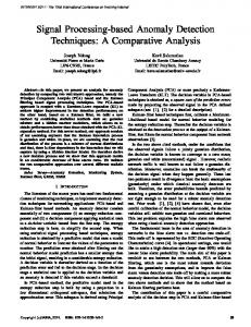
Fig. 1.

Absorption spectrum of NO over the AVIRIS wavelength range.

Since the normalization on  does not matter, we + , G ) ultimately will multiply by the scalar    to obtain a form that is strictly linear in :








 

) ) ) 
 ,   + ,G  + ,G  6  + ,G  IV. E FFECT OF



  C

MODIFIED MATCHED FILTER





(18)

+ ,G ) : + , G ) A  C A





(19) (20)



) 
 ,   + , G A     6 ?  ? A QC ) )  
 ,   + , G A     6 ?  ? A  + , A 
 + , G )   R      6     ? ?A ? ?A
 + , G ) 
 C ? ?A  +-, 
?  ? A   A9?  ? A  ?  ? A9? ? A 6 ?  ? A  :  
 A ?  +N  , ? A
A ? ?A C E    6    A ? ?A ? ?A ? ?A  ) ) )

1 1.5 2 Wavelength (microns)

!#"

$%

 : ? ?A :  ? ? A C




(21) (22) (23)

Then, we can rewrite Eq. (18) as

(24)



&



+ ,G )


./0>! 2&3'4$ ) 8 &   &

(29)

&B6


where A 8  @ is the whitened and meansubtracted background radiance. V. N UMERICAL

EXAMPLES

For the clutter, we have (after some algebraic manipulation)

We illustrate the effect of including the target in the background with some numerical examples. For the clutter, we use hyperspectral radiance data from the AVIRIS sensor [13]. On this scene, we simulate a plume of NO [14] (see Fig. 1). Since this data is in the visible and A near-infrared (VNIR), the plume is necessarily in absorption. If the absorption as a function of wavelength is given by  (plotted in Fig. 1), then the measured radiance in the < th pixel as a function of is given by Beer’s law:

(26)

(30)

From this expression, we have for the signal strength

(25)

and so the signal-to-clutter ratio is given by SCR

(27)

Recall that  is the plume strength at a given pixel, while (defined in Eq. (10)) is a global measure of plume strength across the whole image. The ratio > is a dimensionless value that is independent of overall plume strength. In the strong plume (large ) limit, the SCR in Eq. (27) saturates at



$

This is an upper bound on the SCR that will be obtained for a given plume configuration. Note that as the magnitude of the dimensionless ? ? increases, the limiting signal-to-clutter ratio drops. From the definitions in Eq. (13) and Eq. (19), we can write a more compact expression:

to simplify the following scalar expressions:

 + ,G + , G  + , G

2.5

Fig. 2. The positive curves correspond to the spectra of a dozen points randomly selected from the scene. The negative curve is the plume absorption signal . The radiance in plotted as digital number (DN), and the value shown here corresponds to a plume concentration pathlength of 12.2 ppm-m (parts per million - meters). This is the root mean square plume strength, given by Eq. (10), for our simulated plume.



We introduce “whitened” [12] vectors



0.5



   



  6  ? ? A ? ? ? ?

8>  A SCR
? ?A

A

 A

G)

C

(28)

&

'( &

) &  & =
* &&  & ,+.6 -0/&  6  & '(  & /
*  &   *  & / ('  & 6  &  * &  & 6  *  & /  ('  & 421 5 A 3 * &  & 6  &  *  & / ('  & :  *  & @&
0>! " $&('& ) * &  6 &  '(  & 54  *  &  *  & @ '( &

&

(31) (32)

where . The approximation is accurate if , and is relatively small at wavelengths where is large. In the simulation, we used Eq. (30) directly; the approximation in Eq. (32) was used to obtain the signature vector  used for the matched filters. In
  /  for each wavelength, particular, we take  and then normalize to obtain 
  ?  ? . Fig. 2 shows the spectra from a dozen randomly chosen pixels in this image, and for comparison, the spectrum  .

(.6 &

* & (' & 6 6 

THEILER AND FOY: EFFECT OF SIGNAL CONTAMINATION IN MATCHED-FILTER DETECTION

4

(a)

(b)

(a)

(b)

(c)

(d)

(c)

(d)

(e)

(e)

2

3 sMF uMF cMF actual

Matched filter value

Matched filter value

3

1 0 −1 32 64 96 Horizontal position

%

128

Fig. 3. (a) Broadband image of the hyperspectral dataset, including the simulated (and virtually invisible) plume. (b) Simple matched filter (sMF) image using the plume signature . (c) Uncontaminated matched filter (uMF), , is based on the covariance of the underlying (plume-free) scene. (d) Contaminated matched filter (cMF), , is based on the covariance of the scene with the plume included. (e) Profile of the plume strength (along the line indicated by the stripe across the small image to the left of the plot). The horizontal scale corresponds to position, in pixels, across the image; the vertical scale is based on matched filter values which have been normalized across the whole image to have zero mean and variance equal to unity. Shown are profiles for the simple (sMF), the uncontaminated (uMF), and the contaminated (cMF) matched filters. Also shown is the actual plume profile, scaled so that 1 corresponds to ppm-m.

%

P

P 

%

$ P 





Fig. 3 shows the results of the matched filters applied to the simulated plume imposed on a 128 128 chip from the 
channel AVIRIS image. In fact, there are two plumes; a large plume with a gaussian profile in the center of the image, and a smaller and weaker plume in the upper left corner. The correlation between the spatial structure of the image with the spatial structure of the plume concentration leads, in this case, to ? ?
C . Fig. 3(a) shows a broadband image (sum of all channels) of the data with plume, and in this image, the plume is virtually invisible. The simple matched filter 
I in Fig. 3(b) enhances the plume signature but does not+ suppress , G )  in the background. The optimal matched filter 








 

1 0 −1

0

P
RP   

2

sMF uMF cMF actual

0

32 64 96 Horizontal position

128

Fig. 4. (a) Broadband image of the shuffled scene; these are the same pixels as in Fig. 3, but with a randomized spatial layout. (b) Simple matched filter (sMF). (c) Uncontaminated matched filter (uMF). (d) Contaminated matched filter (cMF); unlike Fig. 3(d), the plume has very little effect on the detectability of the plume. (e) Profile of the matched filter values; unlike Fig. 3(e), the profiles for the uncontaminated (uMF) and contaminated (cMF) matched filters are nearly the same.

Fig. 3(c) suppresses the background considerably, and in that image even the weaker plume is evident in the image. But when the matched filter is based on a covariance computed from data that is contaminated by the plume, as seen in Fig. 3(d), that matched filter is not as effective at suppressing the background; remnants of that background are evident in the image, and the weaker plume is hidden in that background variation. Fig. 3(e) shows a profile across the top of the scene that cuts through the center of the weaker plume. This plot recapitulates the results shown in the images in Fig. 3. One can see the dip in the curve (centroid at horizontal position of 21 pixels) due to the weak plume, but only for the uncontaminated matched filter (uMF) is the dip larger than the fluctuations in the matched filter value due to the background clutter. The dip is also seen in the contaminated matched filter (cMF) profile, but its magnitude is on the same order as the fluctuations due



THEILER AND FOY: EFFECT OF SIGNAL CONTAMINATION IN MATCHED-FILTER DETECTION

to the background. For the simple matched filter (sMF), the profile is completely dominated by the background clutter. As a control experiment, we shuffle the pixels in the image. This way, the mean and covariance of the hyperspectral image cube is strictly preserved, but the plume-scene correlation is C   . Fig. 4 much smaller. For this image, we have ? ?
shows the shuffled image, and the application of the various matched filters to that data. In Fig. 4(d), in contrast to Fig. 3(d), the effect of including the plume in the covariance estimation is much smaller. The plume strength and the spectral statistics of the background clutter (mean and covariance) are the same in both cases. The difference is that the correlation is much smaller for the shuffled image.



2

SCR

10



uMF cMF (shuffled) cMF sMF

1

10

0

0.01 0.02 0.03 0.04 Relative Plume strength

0.05

Fig. 5. Average SCR is plotted against relative plume strength for three different matched filters: simple (sMF), uncontaminated (uCF), and contaminated (cMF). The contaminated matched filter result is plotted for both the original (Fig.
3)
and the shuffled (Fig. 4) image. The relative plume strength is the signal divided by the root mean square of the plume-free image 

 . The vertical line corresponds to the plume trace    strength in Figs. 2-4. The SCR is computed from the matched filter images by first distinguishing the on-plume from off-plume pixels. We define  on as the average value of over the on-plume pixels, and  off is the average over the off-plume pixels. With off is the variance of the matched filter values over the off-plume pixels, then we compute SCR  on  off off .

!  ! $ % P P $

  







P

 

In Fig. 5, we plot the average SCR for matched filter plume detection as a function of relative plume strength. We see that SCR increases with increasing plume strength, but the contaminated matched filters saturate3 at a maximum value. That maximum value is larger for the shuffled image, where the correlation (in particular, the value of ? ? ) is smaller.



VI. C ONCLUSION

+

The band-to-band covariance matrix is altered when the background is linearly contaminated by signal, but the of + G )  effect this contamination on the matched filter 
depends on the correlation between the variation in plume strength over the scene with the variation in the ground spectrum over the scene. The dimensionless vector characterizes this / , the performance of the matched correlation. When ? ?
filter is substantially compromised. We have not investigated typical values of ? ? in practical plume-detection scenarios, but we emphasize that ? ? depends on the plume geometry and profile, not on overall plume strength. Along these lines,

1

we also remark that Eq. (29) indicates that will be relatively small as long as the plume is relatively small compared to the size of the scene. In our example, the plume is relatively large, C . In that scene, with a relative plume strength and ? ?
of four percent, the SCR for the contaminated matched filter was reduced by a factor of 12 compared to the uncontaminated matched filter. A second example, based on shuffling the pixels in the first example, had reduced correlation ( ? ?
C  ) but in other respects was identical to the first example, and in that case the SCR loss was only about 30%.



 






ACKNOWLEDGMENTS The authors are grateful to the Advanced Chemical Identification Technology team for valuable discussions, and to C. Borel for useful comments on the manuscript. R EFERENCES

10

0

5



3 In this simulation, as the plume strength is further increased, we begin to see a decrease in the SCR, due to nonlinearity of the Beer’s Law absorption.

[1] B. R. Foy, R. R. Petrin, C. R. Quick, T. Shimada, and J. J. Tiee, “Comparisons between hyperspectral passive and multispectral active sensor measurements.” Proc. SPIE, vol. 4722, pp. 98–109, 2002. [2] I. S. Reed, J. D. Mallett, and L. E. Brennan, “Rapid convergence rate in adaptive arrays,” IEEE Trans. Aerospace and Electronic Systems, vol. 10, pp. 853–863, 1974. [3] E. J. Kelly, “An adaptive detection algorithm,” IEEE Trans. Aerospace and Electronic Systems, vol. 22, pp. 115–127, 1986. [4] F. C. Robey, D. R. Fuhrmann, E. J. Kelly, and R. Nitzberg, “A CFAR adaptive matched filter detector,” IEEE Trans. Aerospace and Electronic Systems, vol. 28, pp. 208–216, 1992. [5] L. L. Scharf and B. Friedlander, “Matched subspace detectors,” IEEE Trans. Signal Processing, vol. 42, pp. 2146–2156, 1994. [6] D. Manolakis, D. Marden, J. Kerekes, and G. Shaw, “On the statistics of hyperspectral imaging data,” Proc. SPIE, vol. 4381, pp. 308–316, 2001. [7] C. C. Funk, J. Theiler, D. A. Roberts, and C. C. Borel, “Clustering to improve matched filter detection of weak gas plumes in hyperspectral imagery,” IEEE Trans. Geoscience and Remote Sensing, vol. 39, pp. 1410–1420, 2001. [8] J. Theiler, B. R. Foy, and A. M. Fraser, “Characterizing non-Gaussian clutter and detecting weak gaseous plumes in hyperspectral imagery,” Proc. SPIE, vol. 5806, pp. 182–193, 2005. [9] D. Manolakis and G.Shaw, “Detection algorithms for hyperspectral imaging applications,” IEEE Signal Processing Magazine, vol. 19, no. 1, pp. 29–43, 2002. [10] C.-I. Chang, Hyperspectral Imaging: Techniques for Spectral Detection and Classification. New York: Kluwer Academic, 2003. [11] K. Gerlach, “The effects of signal contamination on two adaptive detectors,” IEEE Trans. Aerospace and Electronic Systems, vol. 31, pp. 297–309, 1995. [12] L. L. Scharf, Statistical Signal Processing. Reading, MA: AddisonWesley, 1990, p. 137. [13] AVIRIS (Airborne Visible/Infrared Imaging Spectrometer) Free Standard Data Products, Jet Propulsion Laboratory (JPL), National Aeronautics and Space Administration (NASA). http://aviris.jpl.nasa.gov/html/aviris.freedata.html. [14] A. C. Vandaele, C. Hermans, P. C. Simon, M. Carleer, R. Colin, S. Fally, M. F. Merienne, A. Jenouvrier, and B. Coquart, “Measurements of the NO absorption cross-section from 42000 cm to 10000 cm (2381000 nm) at 220 K and 294 K,” Journal of Quantitative Spectroscopy and Radiative Transfer, vol. 59, pp. 171–184, 1998.





James Theiler received a Ph.D. in Physics from Caltech in 1987, and subsequently held appointments at UCSD, MIT Lincoln Laboratory, Los Alamos National Laboratory, and the Santa Fe Institute. His interests in statistical data analysis and in having a real job were combined in 1994, when he joined the Space and Remote Sensing Sciences Group at Los Alamos. His professional interests include image processing, remote sensing, and machine learning. Bernard R. Foy received a Ph.D. in Physical Chemistry from M.I.T. in 1988 and joined the Chemistry Division at Los Alamos in 1990, where he has worked in lidar and passive infrared chemical sensing, and remote sensing data analysis.