Keywords: input-output system modelling, neural networks, CMAC,
generalization error. Introduction. In system modelling, when there is not enough
information ...
CMAC Neural Network with Improved Generalization Property for System Modelling Gábor Horváth, Tamás Szabó Budapest University of Technology and Economics Department of Measurement and Information Systems Magyar tudósok körútja 2, I. E. 436. H-1111. Budapest, Hungary Tel.: +36 1 463 2677, Fax: +36 1 463 4112, e-mails: {horvath, szabo}@mit.bme.hu
Keywords: input-output system modelling, neural networks, CMAC, generalization error Introduction In system modelling, when there is not enough information to build physical models and where the knowledge available is in the form of input – output data, behavioural (input – output) or black-box modelling approach can be used. In black-box modelling neural networks play important role. Their importance comes from their modelling capability: certain feed-forward neural architectures such as MLPs, RBFs, etc. are universal approximators, which means that a network of proper size can approximate almost any static non-linear input-output mapping with arbitrary accuracy [1], [2]. The static feed-forward architectures can be extended by the addition of local storage elements or by using feedback paths to form dynamic architectures; these dynamic neural structures can be considered as universal devices for modelling non-linear dynamic systems, see e.g. [3], [4], [5]. In certain cases - when the behaviour of the system is changing in time real-time on-line adaptation of the input-output model is required. Real-time adaptation can be reached if the training of the neural network is rather fast. The paper deals with CMAC, a special feed-forward neural architecture. CMAC - which belongs to the family of feed-forward networks with a single linear trainable layer - has some attractive features. The most important ones are its extremely fast learning capability and the special architecture that lets effective digital hardware implementation possible [6], [7], [8]. Although the CMAC architecture was proposed in the middle of the seventies [9] and it has been mentioned as a real alternative of MLP [10], quite a lot open questions have been left even for today. Among them the most important ones are its modelling and generalization capabilities. The modelling capabilities are analysed in some previous works, e.g. in [11] and [12], however the detailed analysis of the generalization error is missing. The results concerning the modelling capability prove that a binary CMAC with onedimensional input can learn any training set exactly, but with multi-dimensional inputs it can learn only such input-output data which come from a function, that is an element of the additive function set. So the modelling capability of the one-dimensional and the multidimensional networks are different. This paper deals with the generalization error of the binary CMAC. The first preliminary results – which show that the generalization error can be rather significant even in onedimensional case if the parameters of the network are not chosen properly - were presented in [13]. The present paper gives a more detailed analysis. It presents a general expression of the
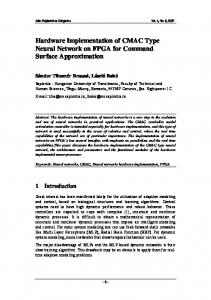
generalization error and gives the derivation of this expression. The paper also gives the real reasons of this significant generalization error: the architecture and the training rule of the network. The modification of the architecture would reduce the implementational advantages of the network, so a modified training rule has to be used to improve the generalization capability. The paper proposes a new training rule, which is based on a new criterion function. The new criterion function has two terms: the first one is the squared error term as usual, the second one is a regularization term, which forces the weights of the network to be as uniformly distributed as possible. The effectiveness of the modified training rule is illustrated by examples. A short overview of the CMAC Cerebellar Model Articulation Controller (CMAC) networks play important role in non-linear function approximation and system modelling. The main advantages of CMAC against MLP, RBF, etc. are its extremely fast learning and the possibility of low-cost digital implementation. This latter property originates from its multiplierless structure and from the fact that it does not require any non-linear function, like the activation function in an MLP. The CMAC network can be considered as an associative memory, which performs two subsequent mappings. The first one - which is a non-linear mapping - projects an input space point u into a binary association vector a. The association vectors always have C active elements, which means that C bits of an association vector are ones and the others are zeros. C is an important parameter of the CMAC network and it is much less than the length of the association vector. (Fig. 1.) ai ai+1 ai+2 ai+3 ai+4 ai+5
u1 u2 u3
discrete input space
u
a
wi wi+1 wi+2 wi+3 wi+4 wi+5
a
C= 4 aj aj+1 aj+2 aj+ 3
y
Σ
y
wj wj+1 wj+2 wj+3
w a association vector weight vector
Fig. 1. The architecture of the binary CMAC network As the value of C affects the generalization property of the CMAC, it is often called generalization parameter. The CMAC uses quantized input, so the number of the possible different input data is finite. There is a one-to-one mapping between the discrete input data and the association vectors, i.e. each possible input point has a unique association vector representation. Every bit in the association vector corresponds to a binary basis function with a finite support of C quantization intervals. This means that a bit will be active if the input value is within the support of the corresponding basis function which support is often called as the receptive field of the basis function. The first mapping should have the following characteristics:
• •
It should map two neighbouring input points into such association vectors, where only a few elements - i.e. few bits - are different. As the distance between two input points grows, the number of the common active bits in the corresponding association vectors decreases. The input points far enough from each other - further then the neighbourhood determined by the parameter C - should not have any common bits. This mapping is responsible for the non-linear property and the generalization of the whole system.
The second mapping calculates the output of the network as a scalar product of the association vector a and the weight vector w: y(u)=a(u) Tw. (1) As the association vector is a binary one, scalar products can be implemented without any multiplication; the scalar product is nothing more than the sum of the weights selected by the active bits of the association vector. y (u) = ∑ wi (2) i : a i ( u ) =1
The two mappings are implemented in a two-layer network architecture. The first mapping can be implemented by a fixed combinational network that contains no adjustable element; the trainable elements, the weight values which can be updated using the simple LMS rule, are in the second layer. The solution of the LMS training can be written in a closed form: w ∗ = A†y d (3)
(
where A † = A T AA T
)
−1
is the pseudoinverse of the association matrix ← A = ← ←
a (1)T a ( 2 )T � ( L )T a
→ → →
(4)
formed from the association vectors and y d T = [ yd (1) yd ( 2) . . . yd ( L ) ] is the output vector formed from the desired values of all training data. The response of the trained network for all possible discrete inputs can be determined using the solution weight vector: y = Tw ∗ = TAT ( AAT ) −1 y d
(
where B = AA
)
T −1
y = TAT B y d
(5) (6)
and T is the matrix formed from all association vectors: 1 0 T = 0 0
1 1 1 1 1 1 1 0 1 1 1 1 1 1 1 1 0 1 1 1 1 1 1 1 � � 0 0 0 0 0 0 ... 0
0 0 1 � 1
0 0 0 0 0 ... 0 0 0 0 0 0 ... 0 0 0 0 0 0 ... 0 1 1 1 1 � 1
(7)
The main results The generalization error The paper shows that the binary CMAC can be regarded as a complex piecewise linear filter, where the elementary filters are arranged in two layers. While the first layer contains one filter, the second layer consists of a filter bank. The characteristics of these filters are determined by the mapping of the first layer of the network (the mapping from the input space into the association vector), the positions of the training data in the input space and the generalization parameter, C. The filter of the first layer is characterised by matrix B that depends only on the positions of the training inputs and the value of C. The elements of the filter bank are specified by TAT . The discrete impulse response of the i-th filter, Gi is the i-th row of TAT . The exact filter representation can be determined if both B and TAT are computed. The analytical expression of B, however, can be determined only for special cases. Such special case is if one-dimensional training input data are used and the input samples are positioned uniformly: the non-linear input-output mapping is sampled uniformly with sampling distance d. Fig. 2 shows the filter representation of the network, for this special case. It must be mentioned, that the filter model is valid not only for this special case, but for all cases. For the general case only the characteristics of the filters will be different. G0
G1
B y
yd
Gd-1
Fig. 2. The filter representation of the binary CMAC This representation is the bases of the derivation of the general expression of the generalization error. For uniformly sampled training data B can be determined:
Bi, j =
n −1
1 ∑ n k =0
2k ( j − i ) 2k ) − 1 cos( n n 2k ( z + 1) 2k (C − zd ) cos + ( zd + d − C ) cos −d n n cos
(8)
C where z = is integer and n is the size of the quadratic matrix, B. The complexity of this d expression is an obstacle of using it easily for analysing the behaviour of the generalization error and for constructing a CMAC with good generalization property. A much more simple form can be reached if z = 1. In this case the (i, i+l)-th element of B can be written as: Bi ,i + l = (− 1)
(l )
1C − r r 2b
l
(9)
where r = C 2 − 4b 2 and b = C − d . Using the results of Eqs. (8) and (9) the relative generalization error, which is the difference between the response of the CMAC and a piecewise linear approximation of the mapping to be learned can be determined analytically. The piecewise linear approximation will give exact responses at the training points and linear interpolation in between. The result for the range of z=1…8 is shown in Fig. 3. 0.2 0.18 0.16 0.14 0.12 0.1 0.08 0.06 0.04 0.02 0
1
2
3
4
5
6
7
8
C/d Fig. 3. The relative generalization error as a function of C/d The figure shows, that the result of a CMAC is exactly the same as the linear interpolation if C/d is integer, i.e the relative generalization error defined before is zero. In the other cases the generalization error can be rather significant. The error can be reduced if larger C is applied, however, too large C will have another effect: the larger the C the smoother the response of the network. This means, that C can be determined correctly only if there is some information about the smoothness of the mapping to be learned. The generalization error for different parameters and different mappings (functions) can be seen in Figs. 4., 5. and 6. c = 8, d= 4
c = 8, d= 7 1.1
1
1 0.9 0.9 0.8 0.8 0.7
0.7
0.6
0.6
0.5
0.5 0.4
0.4
0.3 0.3 0.2 0.2
0.1
0.1 20
40
60
80
100
120
a.)
140
160
180
200
20
40
60
80
100
120
b.)
140
160
180
c = 8, d= 5
1
0.8
0.6
0.4
0.2
0 20
40
60
80
100
120
140
160
180
200
c.) Fig. 4. The response of a CMAC network, trained with a square-wave signal with C = 8 a.) d = 4, b.) d = 7, c.) d = 5 c = 8, d= 5
c = 8, d= 4 140
140
120
120
100
100
80
80
60
60
40
40
20
20
0
0 0
50
100
150
200
250
300
0
50
100
a.)
150
200
250
300
b.) c = 8, d= 7 140
120
100
80
60
40
20
0 0
50
100
150
200
250
300
c.) Fig. 5. The response of a CMAC network, trained with a triangular signal with C = 8 a.) d = 4, b.) d = 7, c.) d = 5 c = 32 , d= 17
c = 32, d= 16
1
1
0.8
0.8
0.6
0.6
0.4
0.4
0.2
0.2
0
0
-0 .2
-0 . 2
-0 .4
-0 . 4
-0 .6
-0 . 6
-0 .8
-0 . 8
-1 0
50
100
150
a.)
200
250
300
-1
0
50
100
150
200
250
300
b.)
Fig. 6. The response of a CMAC network, trained with a sine-wave signal with C = 32 a.) d = 17, b.) d = 16
Modified CMAC learning algorithm The main problem of the LMS training is, that the weights are not evenly incremented which has an effect that the more frequently changed weights can grow much faster than the others and they will dominate the reproduction of the values of the training points. Thus, in the midpoints between the training points, where the less frequently updated - and so the less dominant - weights form the output of the network the error can be large. This effect can be reduced if a modified criterion function is used. The criterion function has two terms. The first one is a usual squared error term. However, there is a new, regularization term, which will be responsible to force the weights selected by an input data to be as similar as possible. The new criterion function is:
(
)
C (k ) = yd (k ) − y (k )
2
λ y (k ) + d − wi (k ) . 2 C 2
(10)
The modified training equation according to the new criterion function is as follows: y (k ) wi (k + 1) = wi (k ) + µ a(k )ε (k ) + λ d − wi (k ) , C
(11)
where the first part is the standard LMS rule for the output layer of the CMAC, and the second part comes from the regularization term. λ is a regularization parameter and the values of µ and λ are responsible for finding a good compromise between the two terms. In Eqs. (10) and (11) wi are the weights that are selected by the active bits of the association vector a(k ) = a(u(k ) ) at the k-th training step. The effect of the modified training rule is illustrated by some examples. Figures 7, 8 and 9 show different situations, where one can compare the responses of the network with the original and the modified training rule. The significant reduction of the generalization error can be seen easily. 220
220
220
200
200
200
180
180
180
160
160
160
140
140
140
120
120
120
100
100
100
80
80
0
50
100
150
200
250
300
0
50
100
a.)
150
200
250
300
80
0
50
100
b.)
150
200
250
300
c.)
Fig. 7. The response of a CMAC network, trained with a square-wave signal a.) � = 1, b.) � = 0, c.) � = 0.5 1
1
1
0.8
0.8
0.8
0.6
0.6
0.6
0.4
0.4
0.4
0.2
0.2
0.2
0
0
0
0
50
100
150
200
250
300
0
50
100
150
200
250
300
0
50
100
150
200
250
a.) b.) c.) Fig. 8. The response of a CMAC network, trained with a half period sine-wave signal a.) � = 1, b.) � = 0, c.) � = 0.5
300
1
1
1
0.8
0.8
0.8
0.6
0.6
0.6
0.4
0.4
0.4
0.2
0.2
0.2
0
0
0
−0.2
−0.2
−0.2
−0.4
−0.4
−0.4
−0.6
−0.6
−0.6
−0.8
−0.8
−1
0
50
100
150
200
250
300
−1
−0.8
0
50
100
150
200
250
300
−1
0
50
100
150
200
250
300
a.) b.) c.) Fig. 9. The response of a CMAC network, trained with a higher-frequency sine wave signal a.) � = 1, b.) � = 0, c.) � = 0.5 Conculsion This paper studies the generalization properties of the CMAC neural network. The importance of the network comes from its special architecture and from its fast training. The architecture of CMAC is especially suitable for simple digital hardware implementation, so this network is a good candidate for applications where low cost embedded solution and high-speed operation with real-time online adaptation are required, e.g. in smart sensors, in measuring systems, etc. The paper gives detailed analytical results on the generalization error. It gives a new filterbank representation of the network and an analytical expression of the generalization error for one-dimensional case. As the real reason of the rather poor generalization property has been recognised a modified training rule could be developed which greatly reduces the generalization error. The extension of the analytical results for multidimensional cases will be the task of the near future. References [1]
Cybenko, G. "Approximation by superpositions of a sigmoidal function" Mathematics of Control, Signals and Systems, vol. 3. pp. 303-314, 1989.
[2]
Park, J. - Sandberg, I.W. "Approximation and Radial-Basis-Function Networks", Neural Computation, Vol 5. pp 30516., 1993.
[3]
Narendra, K.S. - Pathasarathy, K. (1991) "Identification and Control of Dynamic Systems Using Neural Networks", IEEE Trans. on Neural Networks, Vol. 2. pp. 252-262.
[4]
Haykin, S. "Neural Networks A Comprehensive Foundation", Macmillan College Publishing Co., New York, 1994.
[5]
IEEE Transactions on Neural Networks, Special Issue on Dynamic Recurrent Neural Networks: Theory and Applications, Vol. 5. No. 2. March, 1994.
[6]
Miller, T. W. Box, B. A. and Whitney, E. C. "Design and implementation of a high-speed CMAC neural network using programmable CMOS logic cell arrays" Univ. of New Hampshire, Rept. no. ECE.IS.90.01., 1990.
[7]
Horváth, G. and Deák, F. "Hardware Implementation of Neural Networks Using FPGA Elements" Proc. of The International Conference on Signal Processing Application and Technology, Santa Clara Vol. II. pp. 60-65. 1993.
[8] Szabó, T. and Horváth, G.: "CMAC and its Extensions for Efficient System Modelling", International Journal of Applied Mathematics and Computer Science, 1999. Vol. 9. No. 3. pp. 571-598. [9]
Albus, J. S. "A New Approach to Manipulator Control: The Cerebellar Model Articulation Controller (CMAC)", Transaction of the ASME, Sep. 1975. pp. 220-227.
[10] Miller, T. W. III. Glanz, F. H. and Kraft, L. G. "CMAC: An Associative Neural Network Alternative to Backpropagation" Proceedings of the IEEE, vol. 78. No. 10. Oct. 1990. pp. 1561-1567. [11] Brown, M. - Harris, C. J. and Parks, P. "The Interpolation Capability of the Binary CMAC", Neural Networks, Vol. 6. No. 3. 1993. pp. 429-440. [12] Brown, M. and Harris, C. J.: "Neurofuzzy adaptive modelling and control" Prentice Hall, New York, 1994. [13] Szabó, T. and Horváth, G. "Improving the generalization capability of the binary CMAC” Proc. of the International Joint Conference on Neural Networks, IJCNN’2000. Como, Italy, Vol. 3, pp. 85-90.