This paper describes how to use the Matlab software package CMregr, and also gives some limited information on the CM-estimation problem itself. For detailed ...
CMregr – A Matlab software package for finding CM-Estimates for Regression Ove Edlund Lule˚ a University of Technology, Department of Mathematics, S-97187 Lule˚ a, Sweden
1
Introduction
This paper describes how to use the Matlab software package CMregr, and also gives some limited information on the CM-estimation problem itself. For detailed information on the algorithms used in CMregr as well as extensive testings, please refer to (Arslan, Edlund & Ekblom 2002) and (Edlund & Ekblom 2002). New methods for robust estimation regression have been developed during the last decades. Two important examples are M-estimates (Huber 1981) and S-estimates (Rousseeuw & Yohai 1984). A more recent suggestion is Constrained M-estimates – or CM-estimates for short – where the good local properties of the M-estimates and good global robustness properties of the S-estimates are combined (Mendes & Tyler 1995). CM-estimates maintain an asymptotic breakdown point of 50% without sacrificing high asymptotic efficiency. Until recently, there was no satisfying method for fast computation of CMestimates, with high precision. The Matlab code CMregr presented here is an implementation of a new algorithm for CM-estimates for regression presented in (Arslan et al. 2002) and (Edlund & Ekblom 2002), that addresses these issues. We can formulate CM-estimation for regression in the following way. Consider the linear model y = X β + e, where y = (y1 , y2 , ..., yn )T is the response vector, X is an (n × p) design matrix, β a p-dimensional vector of unknowns and e = (e1 , e2 , ..., en )T the error vector. Alternatively we may write yi = xTi β + ei ,
i = 1, 2, ..., n
where xi is the i:th row in X. Define the residuals as ri = yi − xTi β, i = 1, 2, ..., n. The CM-estimation problem is to find the global minimum of n
L(β, σ) = c
1X ρ(ri /σ) + log σ n i=1 1
(1)
over β ∈ Rp and σ ∈ R+ subject to the constraint n
1X ρ(ri /σ) ≤ ε ρ(∞) n i=1
(2)
Here ρ(t) is a bounded function, symmetric around zero and nondecreasing for t ≥ 0, and c and ε are tuning parameters that need to be chosen carefully, as described in Section 2. If strict inequality holds in the constraint above we get the redescending M-estimating equations for β and σ. Equality in the constraint instead gives the S-estimate, where σ is minimized with respect to (2). The reason is that for equality constraint we have L(β, σ) = constant + log(σ), which is minimized by minimizing σ. Thus the S- and CM-estimates are closely related. However, the CM-estimates have some nice properties not shared by the S-estimates as exemplified in Section 2. Two ρ-functions are considered in this paper: Tukey biweight ( 2 4 6 t − t2 + t6 , for |t| ≤ 1 2 ρ(t) = 1 , for |t| > 1 6 and Welsh
1 2 ρ(t) = (1 − e−t ) . 2 In CMregr these two functions are referred to as tukey and welsh respectively. As shown in Section 5, it is easy to add customized ρ-functions to CMregr, to calculate other CM-estimates.
2
Estimation parameters and how to choose them
The parameters c and ε in (1) and (2) are used for tuning the CM-estimates. The parameter ε controls the asymptotic breakdown point: The asymptotic breakdown point is given by min(ε, 1 − ε). By choosing ε = 0.5, the highest possible asymptotic breakdown point is achieved. No other choice is sensible when CM-estimates are considered. This means that the only parameter that really matters for CM-estimates is c. If c is small, the S-estimate for ε = 0.5 is found rather than an CMestimate. For normally distributed residuals, it is in general required that c > 15 (Tukey) and c > 5.3 (Welsh) to get a CM-estimate rather than an S-estimate. The properties of the estimate varies with c. Mendes & Tyler (1995) made a theoretical investigation of the asymptotic relative efficiency, and the residual gross error sensitivity: γr∗ . When those results are applied to Tukey biweight and Welsh, it is revealed that the sensitivity γr∗ has a minimum for some c, and that the efficiency is an increasing function of c. This implies that it is pointless to choose c smaller than the minimizer of γr∗ , but it may 2
be worthwhile to choose a greater value. For Tukey, γr∗ is minimized by c = 19.62, and for Welsh the minimizer is c = 7.348. Other possible choices are given in Table 1. Table 1: Asymptotic relative efficiency and residual gross error sensitivity (γr∗ ) for varying choices of c in Tukey biweight and Welsh CM-estimates.
Tukey biweight c 19.62 22.57 28.97 41.68 56.02
eff 0.847 0.900 0.950 0.980 0.990
Welsh
γr∗ 1.64 1.66 1.77 2.01 2.28
c 7.348 8.930 12.07 18.39 25.54
eff 0.838 0.900 0.950 0.980 0.990
γr∗ 1.58 1.61 1.73 2.02 2.31
The table for Tukey biweight in (Mendes & Tyler 1995) looks different since they use a slightly modified ρ-function in their analysis. The values in Table 1 hold for tukey and welsh in CMregr. It is possible to use CMregr for finding S-estimates by setting c = 0. Then the properties of the estimate are controlled by changing the asymptotic breakdown point ε. As a comparison, Table 2 shows the values of ε corresponding to Table 1, with the addition of ε = 0.5. A table for Tukey biweight with some more reasonable choices of ε can be found in (Rousseeuw & Yohai 1984). Table 2: Asymptotic relative efficiency for varying choices of asymptotic breakdown point ε in Tukey biweight and Welsh S-estimates.
Tukey biweight ε 0.5000 0.2001 0.1638 0.1194 0.0786 0.0570
Welsh
eff 0.287 0.847 0.900 0.950 0.980 0.990
ε 0.5000 0.1835 0.1400 0.0963 0.0596 0.0417
eff 0.289 0.838 0.900 0.950 0.980 0.990
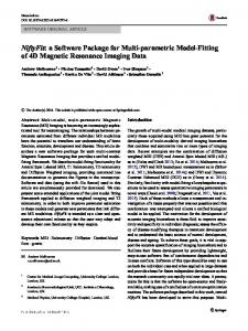
Figure 1 illustrates the difference in efficiency between some estimates with breakdown point 0.5, and least squares. High efficiency means that the regression line is close to the least squares solution if there are no outliers. In Figure 2 we see the price one has to pay in S-estimates to get the same asymptotic relative efficiency as in CM-estimates. In the right graph of Figure 2, the S-estimate “breaks down” when one more outlier is added compared to the left graph. This is because of the very low breakdown point required for S-estimates to get high efficiency. 3
120
LS S, ε = 0.5 CM, c = 19.62 CM, c = 28.97
100
80
60
40
20
0 0
10
20
30
40
50
60
70
80
90
100
Figure 1: Regression lines for least squares (LS), S-estimate with ε = 0.5 and CM-estimates with c = 19.62 and c = 28.97 using Tukey biweight.
45 40
LS S CM
45 40
35
35
30
30
25
25
20
20
15
15
10
10
5
5
0 0
10
20
30
40
50
0 0
60
LS S CM
10
20
30
40
50
60
Figure 2: Regression lines for least squares (LS), S-estimate with ε = 0.1194 and CM-estimate with c = 28.97 using Tukey biweight. Both parameters correspond to an asymptotic efficiency of 0.95.
4
c = 19.62, Inliers = 35, Outliers = 27 (43.5 %)
c = 28.97, Inliers = 35, Outliers = 27 (43.5 %)
45
45
40
40
35
35
30
30
25
25
20
20
15
15
10 5 0 0
10
LS CM 1, obj = 3.818 CM 2, obj = 4.318 10
20
LS CM 1, obj = 4.598 CM 2, obj = 4.558
5
30
40
50
0 0
60
10
20
30
40
50
60
Figure 3: Regression lines for least squares (LS), and for the two local minima of the CM-estimate with c = 19.62 in the left graph, and with c = 28.97 in the right graph, using Tukey biweight. The values of the corresponding objective functions (1) are in the label box. c = 28.97, Inliers = 35, Outliers = 34 (49.3 %) 45 40 35 30 25 20 15 10 5 0 0
LS CM 1, obj = 4.304 CM 2, obj = 4.468 10
20
30
40
50
60
Figure 4: Regression lines for least squares (LS), and for the two local minima of the CM-estimate with c = 28.97, using Tukey biweight. The values of the corresponding objective functions (1) are in the label box.
The optimization problem of finding the CM-estimates shares the property, that there may be a few local minima, with the S-estimates. Figure 3 shows the two local minima for CM with two choices for the parameter c. The data-sets are the same in the two graphs with 43.5% outliers in the data. The right graph has the greater c corresponding to a higher efficiency, but then the objective function (1) reports the “wrong” solution as the best one. The CM-estimate has an asymptotic 50% breakdown point, but that is not achieved in this case. This is what can be expected when the “good data” is too scattered. Figure 4 shows that for better behaved “good data”, the 50% breakdown point is achieved, even for greater values of c. It is however obvious that the observed breakdown point may drop a bit. And the drop is generally greater for CM-estimates with higher efficiency.
5
3
The algorithm
The CM-estimates cannot be expressed explicitly. Computing these estimates numerically is a challenging problem, since we like to minimize an objective function where many local minima may exist. If σ is held fixed in (1), we have a linear model M-estimation problem. The algorithms in (Arslan et al. 2002) and (Edlund & Ekblom 2002) make use of the fact that very good algorithms exist for this problem (Edlund 1997). So the solution is found by solving a series of linear model M-estimation problems. The updating of σ is done as a separate step, that requires much less calculations, since we have a one-dimensional problem at hand. Details on this issue is found in (Edlund & Ekblom 2002). To find the global minimum, good starting points for the local iteration above is generated by considering many subsamples with p observations (Arslan et al. 2002).
4
Invoking the software
There are two commands in CMregr for calculating CM-estimates: globalCMregr and localCMregr. The first of these tries to find the “global minimum” using the technique described above, while localCMregr needs a user-supplied starting point.
globalCMregr [β, σ, stat] = globalCMregr(ρ-fun, c, ε, X, y) or [β, σ, stat] = globalCMregr(ρ-fun, c, ε, X, y, iters) Input parameters ρ-fun c ε X y iters
– – – – – –
the chosen ρ-function as a Matlab string e.g. ’tukey’ or ’welsh’. the tuning parameter, from Table 1. asymptotic breakdown point. Always use 0.5 for CM-estimates. the design matrix. the response vector. the number of subsamples to investigate for a good starting point. If this is omitted, the routine makes a guess of the number of subsamples to use.
6
Output parameters β & σ – the calculated solution. stat – some additional data on the solution. stat.border is 1 if the solution fulfills (2) with equality, and 0 if (2) is fulfilled with strict inequality. stat.obj is the value of the objective function (1) at the solution. stat.constr is the difference between the left and right hand sides of (2). Example Let us define a design matrix and a response vector: >>X = [1 0;1 1;1 3;1 4;1 8] X = 1 0 1 1 1 3 1 4 1 8 >>y = [1 2 3 4 0.5]’; The Tukey biweight CM-estimate with c = 19.62 (see Table 1) is then found by >>[b,s,stat] = globalCMregr(’tukey’,19.62,0.5,X,y) b = 1.07973997179869 0.71013001410066 s = 0.54750922628337 stat = border: 0 obj: 0.63014080945719 constr: -0.02051392582918 Since stat.border = 0, the solution is in the interior of the feasible region, i.e. (2) is not fulfilled with equality. If the number of outliers would increase, the solution would eventually reach the border. In a sense one could say that, if outliers are plentiful, the S-estimate kicks in and saves the day. Plotting the regression line yields: >>t = -1:9; >>plot(X(:,2),y,’o’,t,b(1)+b(2)*t)
7
8
7
6
5
4
3
2
1
0 -1
0
1
2
3
4
5
6
7
8
9
localCMregr [β, σ, stat] = localCMregr(ρ-fun, c, ε, X, y, βstart ) Input parameters ρ-fun c ε X y βstart
– – – – – –
the chosen ρ-function as a Matlab string e.g. ’tukey’ or ’welsh’. the tuning parameter, from Table 1. asymptotic breakdown point. Always use 0.5 for CM-estimates. the design matrix. the response vector. the initial guess of the solution β. The algorithm searches from this point and finds a local minimum.
Output parameters β & σ – the calculated solution. stat – some additional data on the solution. stat.border is 1 if the solution fulfills (2) with equality, and 0 if (2) is fulfilled with strict inequality. stat.obj is the value of the objective function (1) at the solution. stat.constr is the difference between the left and right hand sides of (2). Example Using the same design matrix and response vector as in the previous example, we want to calculate the Welsh estimate with c = 12.07 (see Table 1) and starting from the least squares solution: >>[b,s,stat] = localCMregr(’welsh’,12.07,0.5,X,y,X\y) b = 2.28257700557494 -0.07363502459208 s = 4.06413162024954 8
stat = border: 0 obj: 1.94453719549732 constr: -0.20506734889203 Also in this example the solution is in the interior of the feasible region (stat.border = 0). Plotting the solution yields: 4
3.5
3
2.5
2
1.5
1
0.5 -1
0
1
2
3
4
5
6
7
8
9
The badly chosen starting point results in a solution that is a local minimum, and not the global minimum we were interested in.
5
Adding customized ρ-functions
The ρ-functions that are supplied with CMregr are implemented as Matlabfunctions. This means that it is quite easy to add new ones manually. The Matlab-function that implements the ρ-function must obey the following rules: 1. If the Matlab-function is called with one vector as input, it should return a vector with the ρ-function applied to each element in the input vector. Example: >>welsh([-1 0 1 2]) ans = 0.3161 0
0.3161
0.4908
2. If the vector is followed by the parameter 0 (zero), the same vector as above should be returned. Example: >>welsh([-1 0 1 2],0) ans = 0.3161 0
0.3161
0.4908
3. If the vector is followed by the parameter 1, the Matlab-function should return a vector with the derivative ρ0 applied to each element in the input vector. Example: >>welsh([-1 0 1 2],1) ans = -0.3679 0
0.3679 9
0.0366
4. If the vector is followed by the parameter 2, the Matlab-function should return a vector with the second derivative ρ00 applied to each element in the input vector. Example: >>welsh([-1 0 1 2],2) ans = -0.3679 1.0000
-0.3679
-0.1282
The routines in CMregr make use of all these four cases. This puts some restrictions on what ρ-functions can be used. The ρ-function has to be twice differentiable! The code for the welsh function of CMregr serves as an example of how to implement such a function, and may serve as a template for customized ρ-functions in CMregr: function v = welsh(r,diff) if nargin==1 diff = 0; elseif nargin∼ =2 error(’Wrong number of input arguments’) end switch diff case 0 v = 0.5*(1–exp(–r.∧ 2)); case 1 v = r.*exp(–r.∧ 2); case 2 r2 = r.∧ 2; v = (1–2*r2).*exp(–r2); otherwise error(’Illegal order of differentiation’) end
References Arslan, O., Edlund, O. & Ekblom, H. (2002), ‘Algorithms to compute CMand S-estimates for regression’, Metrika 55, 37–51. Edlund, O. (1997), ‘Linear M-estimation with bounded variables’, BIT 37(1), 13–23. Edlund, O. & Ekblom, H. (2002), Constrained M-estimates for regression – and how to compute them. Manuscript in preparation. Huber, P. (1981), Robust Statistics, John Wiley, New York.
10
Mendes, B. & Tyler, D. E. (1995), Constrained M-estimates for regression, in ‘Robust Statistics; Data Analysis and Computer Intensive Methods’, Vol. 109 of Lecture Notes in Statistics, Springer, New York, pp. 299–320. Rousseeuw, P. J. & Yohai, V. J. (1984), Robust regression by means of Sestimators, in J. Frank, W. H¨ardle & R. D. Martin, eds, ‘Robust and Nonlinear Time Series Analysis’, Lecture Notes in Statistics, Springer, New York, pp. 256–272.
11