Mar 26, 2013 ... Game Animation: Most computer games revolve around characters ... Producing
natural looking animation is the topic of our next few lectures.
CMSC 425
Dave Mount
CMSC 425: Lecture 13 Animation for Games: Basics Tuesday, Mar 26, 2013 Reading: Chapt 11 of Gregory, Game Engine Architecture. Game Animation: Most computer games revolve around characters that move around in a fluid and continuous manner. Unlike objects that move according to the basic laws of physics (e.g., balls, projectiles, vehicles, water, smoke), the animation of skeletal structures may be subject to many complex issues, such as physiological constraints (how to jump onto a platform), athletic technique (how a basketball player performs a lay-up shot or a warrior hurls a spear), stylistic choices (how a dancer moves), or simply the arbitrary conventions of everyday life (how a person steps out of a car or how a dog wags its tail). Producing natural looking animation is the topic of our next few lectures. Image-based Animation: Most character animation arising in high-end 3-dimensional computer games is based on skeletal animation. Prior to this, most animation was based on two-dimensional methods. Cel Animation: Before the advent of computers, the standard method of producing animation in films was by a process where an artist would paint each individual frame of a characters animation on a transparent piece of celluloid, which would then be placed over a static background. The term celluloid was shortened to cel. Given the need to generate 30 or 60 frames per second, this is a very labor-intensive process. Often a master animator would sketch a sparse set of key drawings or key frames showing the most important transitions, and then less experienced artists would add color and fill in intermediate frames. The process of inserting intermediate drawings in between the key frames acquired the name of tweening. This approach has been extended to computer animation, where the modeling software generates a complete representation of certain key frames and some type of interpolation is then applied to generate the intermediate frames. Sprites: An early adaptation of the cel approach to computer games is called sprite animation, where a series of bit-map images is generated (see Fig. 1(a)). Sprites were typically generated to form a cycle so that the sequence could be played repeatedly to generate the illusion of walking or running.
(a)
(b)
Fig. 1: Image-based animation: (a) sprites and (b) a control mesh for morphing. Animated Textures: A simple extension of sprites, used even in modern games for low resolution models, is to model a moving object by a sequence of images, which are played back in a loop. Lecture 13
1
Spring 2013
CMSC 425
Dave Mount This could be used, for example, to show trees swaying in the distance or background crowd motion in a sports arena.
Texture Morphing: Storing a large number of large animated textures can be wasteful in space. One way of saving space is to store a small number of key images and transition smoothly between them. In computer graphics, morphing refers to the process of continuously mapping one image into another through a process of gradual distortion. This is typically done by selecting a small set of corresponding control points on each of the two images. For example, to morph between two faces these might consist of the corners of the mouth, nose, eyes, ears, chin, and hairline. Next, a pair of compatible control meshes is generated, one for each image (see Fig. 1(b)). (A good choice would be a Delaunay triangulation, as discussed in Lecture 9.) Then, the animation process involves linearly interpolating between these two images. Skeletal Models: As mentioned above, the most common form of character animation used in high-end 3-dimensional games is through the use of skeletal animation. A character is modeled as skin surface stretched over a skeletal framework which consists of moving joints connected by segments called bones (see Fig. 2). The animation is performed by modifying the relationships between pairs of adjacent joints, for example, by altering joint angles. We will discuss this process extensively later.
Fig. 2: Skeletal model. A skeletal model is based on a hierarchical representation where peripheral elements are linked as children of more central elements. Here is an example: Root (whole model) . Pelvis . . . Spine . . . . . Neck . . . . . . Head . . . . . Right shoulder . . . . . . Right elbow . . . . . . . Right hand . . . . . Left shoulder . . . . . . Left elbow . . . . . . . Left hand . . . . Right thigh . . . . . Right knee . . . . . . Right ankle . . . . Left thigh
Lecture 13
2
Spring 2013
CMSC 425
Dave Mount . .
. .
. .
. .
. .
Left knee . Left ankle
Clearly, a skeletal model can be represented internally as a multi-way rooted tree, in which each node represents a single joint. The bones of the tree are not explicitly represented, since (as we shall see) they do not play a significant role in the animation or rendering process. We will discuss later how the skin is represented. For now, let us consider how the joints are represented. Joint representation: At a minimum, we need to be able to perform the following operations on any skeleton tree: enumerate(): Iterate through all the joints in the skeleton. In some implementations this might need to be done according to a particular tree traversal (preorder or postorder). For the algorithms we will discuss later, the order of enumeration will not be significant. isRoot(j): Return true if j is the root node and false otherwise. parent(j): For a given non-root node j, return its parent, which we denote by p(j). Depending on the details of the algorithms involved, it may also be useful to access a joint’s children, but we will not need this. Given the above requirements, the tree can be represented very simply as an array of triples, where each triple consists of: • a name for the joint (which will be useful for debugging), • a structure holding the joint’s internal information (which we describe below), and • the index of the joint’s parent in this array. We can make the convention of storing the root joint in index 0 of this array, and therefore we can detect the root node easily. Of course, this is just one possible representation. What does the joint’s “internal information” consist of? Each joint can be thought of as defining its own joint coordinate frame (see Fig. 3(a)). Recall that in affine geometry, a coordinate frame consists of a point (the origin of the frame) and three mutually orthogonal unit vectors (the x, y, and z axes of the frame). These coordinate frames are organized hierarchically according to the structure of the skeleton (see Fig. 3(b)). Rotating a joint can be achieved by rotating its associated coordinate frame. Each frame of the hierarchy is understood to be positioned relative to its parent’s frame. In this way, when the shoulder joint is rotated, the descendent joints (elbow, hand, fingers, etc.) also move as a result (see Fig. 3(c)). Clearly, in order to achieve this effect, we need to know the relationships between the various joints of the system. A basic fact from affine geometry is that, given any two coordinate frames in ddimensional space, it is possible to convert a point represented in one coordinate frame to its representation in the other frame by multiplying the point (given as a (d + 1)-dimensional vector in homogeneous coordinates) times a (d + 1) × (d + 1) matrix. Let’s imagine that we are working in 3-dimensional space. For any two joints j and k, let T[k←j] denote the change of coordinates transformation that maps a point in joint j’s coordinate system to its representation in k’s coordinate system. That is, if v is a column vector in homogeneous coordinates representing of a point relative to j’s coordinate system, then v ′ = T[k←j] · v is v’s representation relative to k’s coordinate frame. Given any non-root joint j, recall that p(j) denotes its parent joint. Let M denote the root of the tree, which is associated with the entire skeletal model. We are interested in the following transformations: Lecture 13
3
Spring 2013
CMSC 425
Dave Mount
j4
j0 j5 j1
j2
j3
j4
j1
j2
j3
j1
j2
j3
j5 30◦
j4 j0
j0 j5
(a)
(b)
(c)
Fig. 3: Skeletal model. Local-pose transformation: T[p(j)←j] converts a point in j’s coordinate system to its representation in its parent’s coordinate system. Inverse local-pose transformation: T[j←p(j)] converts a point in j’s parent’s coordinate system to j’s coordinate system. Clearly, T[j←p(j)] = (T[p(j)←j] )−1 . Which of these transformation matrices is associated with the joint? It turns out to be neither. We shall see that there is yet another matrix that is more important. (Well, there is another matrix more important at least for the purposes of the skin rendering algorithm that we shall describe later. You may have your own reasons for storing one or both of these matrices, since they are certainly relevant to the local processing of the skeleton.) Storing local-pose transformations: If you wanted to store these matrices, how would you do so? As mentioned above, they can be represented as matrices, either a 3 × 3 for 2-dimensional animations or a 4 × 4 for 3-dimensional animations. You may prefer to use an alternative representation, depending on your application. For example, if you working in 2-dimensional space, then the transformation T[j←p(j)] most likely consists of two components, a rotation angle θ, that aligns the two x-axes, and a translation vector vt from p(j)’s origin to j’s origin. This is a more concise representation. Storing a 3 × 3 matrix involves storing 9 floats, whereas storing the pair (θ, vt ) involves only 3 floats. Given this concise representation, it is easy to derive the inverse as the pair (−θ, −vt ). Also, it is easy to derive the associated matrices from this representation. (We will skip this easy exercise in affine geometry, since we haven’t discussed affine geometry in detail.) Is there a similarly concise representation for the local-pose transformation in 3-dimensional space? The answer is yes, but the issue of rotation is more complicated. Again, in order to represent T[j←p(j)] , you need to store a 3-dimensional rotation and a translation. The translation vector vt can be stored as a 3-dimensional vector. However, how do you represent rotations in three dimensional space? There are two common methods: Euler angles: It turns out that any rotation in 3-dimensional space can be expressed as the composition of three rotations, one about the x-axis, one about the y-axis, and one about the z-axis. These are sometimes referred to as pitch, roll, and yaw (see Fig. 4).
Lecture 13
4
Spring 2013
CMSC 425
Dave Mount
z
x
φ Pitch
z
y
z
x
θ Roll
y
ψ
y
x Yaw
Fig. 4: Rotations by Euler angles. Quaternions: While Euler angles are easy for humans to work with, they are not the most mathematically elegant manner of representing a rotation. Why this is so is rather hard to explain, but as an example of why, consider the question of how to interpolate between two Euler angle rotations. Suppose that one is represented by the rotations (φ0 , θ0 , ψ0 ) and the other by (φ1 , θ1 , ψ1 ). In order to generate a smooth interpolation between these two rotations, you would naturally consider performing a linear interpolation � between them. For example, the midpoint rotation would 1 θ0 +θ1 ψ0 +ψ1 be given by φ0 +φ , , . If you would do so (and trust me on this), you would find 2 2 2 this midpoint rotation would not appear to look anything close to the initial or final rotations. There is, however, a mathematically clean solution to the representation of 3-dimensional angles, which is called a quaternion. This is a mathematical object that was discovered around 150 years ago by the Irish mathematician Hamilton. It would take too long to explain how quaternions work, but in a nutshell, a quaternion represents a 3-dimensional rotation by a 4-element vector. (Note that this is less space efficient than Euler angles, which require only 3 numbers, but the 4-element vector is of unit length, so it is possible to derive the 4th component from the first 3.) There is a multiplication operator defined on quaternions, and it is possible to compose two rotations by multiplying the associated quaternions. One nice feature of quaternions is that, unlike Euler angles, they interpolate nicely. Because a quaternion is a unit vector, you need to be sure to use spherical interpolation (that is, interpolating along great circle arcs) rather than linear (straight-line interpolation). The good news is that, without understanding the mathematical details of quaternions, it is possible to download software that will do all of this for you. So, the upshot of this is that you can store the local pose transformation using either 6 or 7 floats (a rotation stored as 3 Euler angles or 4 quaternion coefficients) and a 3-element translation vector. As in the 2-dimensional case, there are easy procedures for computing the inverse transformations from either representation. Bind Pose: Before discussing animation on skeletal structures, it is useful to first say a bit about the notion of a pose. In a typical skeleton, joints move by means of rotations. (It is rather interesting to think about how this happens for your own joints. For example, your shoulder joint as two degrees of freedom, since it can point your upper arm in any direction it likes. Your elbow also has two degrees of freedom. One degree comes by flexing and extending your forearm. The other can be seen when you turn your wrist, as in turning a door knob. Your neck has (at least) three degrees of freedom, since, like your shoulder, you can point the top of your head in any direction, and, like your elbow, you can also turn it clockwise and counterclockwise.) Assigning angles to the various joints of a skeleton (and, more generally, specifying the local pose Lecture 13
5
Spring 2013
CMSC 425
Dave Mount
transformations for each joint) defines the skeleton’s exact position, that is, its pose. When an designer defines the initial layout of the model’s skin, the designer does so relative to a default pose, which is called the reference pose or the bind pose. For human skeletons, the bind pose is typically one where the character is standing upright with arms extended straight out to the left and right (similar to Fig. 2 above). There are two important change-of-coordinate transformations for this process. Bind-pose transformation: (also called the global pose transformation) T[M ←j] converts a point in j’s coordinate system to its representation in the model’s global reference coordinate system M . We can express the matrix associated with this transformation as the product of the matrices associated with the local pose transformations from j up to the root. In particular, suppose that the path from j to the root is j = j1 → j2 → . . . → jm = M , then (assuming postmultiplication, as OpenGL does) the bind-pose transformation is T[M ←j] = T[jm ←jm−1 ] . . . T[j3 ←j2 ] T[j2 ←j1 ] =
m−1 Y
T[jm−i−1 ←jm−i ] .
i=1
This transformation is important since, if we know of a point’s position relative to its nearest joint (for example, a point on the tip of the index finger), this transformation allows us to convert this point into its representation in the model’s global coordinate frame. In spite of this obvious usefulness, we shall see that the inverse of this transformation, given next, is even more important. Inverse bind-pose transformation: T[j←M ] converts a point in the model’s global coordinate system to its representation relative to j’s local coordinate system. Clearly, T[j←M ] = (T[p(j)←j] )−1 . Equivalently, T[j←M ] = T[j1 ←j2 ] T[j2 ←j3 ] . . . T[jm−1 ←jm ] =
m−1 Y
T[ji ←ji+1 ] .
i=1
When an artist places the skin on an object, he/she is implicitly associating a triangulated mesh with the skeleton. The modeling software knows the coordinates of the vertices of this mesh with respect to the model’s global coordinate system. However, in order to know how each vertex will respond to changes in joint angles, we will need to map each vertex of the mesh into its representation local to one or more nearby joints. Next time, we will discuss the process of how to render skin on an animated skeleton. We shall see that the most relevant of all the transformations associated with any joint is the inverse bind-pose transformation, which indicates how to map a vertex from the global frame down to a local frame. So, we can now answer the question raised earlier, “What does the joint’s internal information consist of?” The answer is the inverse bind-pose transformation. Next time, we’ll see exactly why.
Lecture 13
6
Spring 2013


![[PDF] Download Basics Animation 02: Digital Animation Top Ebook ...](https://m.moam.info/img/260x300/pdf-download-basics-animation-02-digital-animation_647808dd097c474e708c5d92.jpg)