Co-Evolutionary Learning on Noisy Tasks Paul J. Darwen Cognitive Science Research Group Department of Computer Science and Electrical Engineering The University of Queensland Brisbane, Queensland 4072 Australia
[email protected]
Jordan B. Pollack DEMO Laboratory Computer Science Department Volen National Center for Complex Systems Brandeis University Waltham, Massachusetts 02454-9110 USA
[email protected]
AbstractThis paper studies the effect of noise on coevolutionary learning, using Backgammon as a typical noisy task. It might seem that co-evolutionary learning would be ill-suited to noisy tasks: genetic drift causes convergence to a population of similar individuals, and on noisy tasks it would seem to require many samples (i.e., many evaluations, and long computation time) to discern small differences between similar population members. Surprisingly, this paper learns otherwise: for small population sizes, the number of evaluations does have an effect on learning; but for sufficiently large populations, more evaluations do not improve learning at all — population size is the dominant variable. This is because a large population maintains more diversity, so that the larger differences in ability can be discerned with a modest number of evaluations. This counter-intuitive result means that coevolutionary learning is a feasible method for noisy tasks, such as military situations and investment management.
tion 2.1 looks at the effects of noise on co-evolutionary learning. Section 3 describes a co-evolutionary learning system for the game of Backgammon. Section 4 discusses the results on how population size and the number of evaluations affect learning performance. The paper concludes in Section 5.
1 Introduction Co-evolutionary learning can discover solutions to problems, without knowledge from human experts. The method has achieved impressive results on simple games such as the iterated Prisoner’s Dilemma [1] [2] [3] [5] [15], and on other non-game tasks, such as creating a sorting algorithm [10]. Although noise and evolutionary computation have been looked at [4] [19], past work on co-evolution has often studied tasks that were noise-free or nearly so, with few exceptions [12]. Practical applications are notoriously noisy, such as military simulations [6] and investment portfolio management [17] [18]. This paper studies the effects of noise on co-evolutionary learning, with the game of Backgammon (which uses dice) as a learning task. We are not particularly interested in Backgammon itself, but it makes a convenient test problem. The lessons learned from Backgammon are applicable to realworld noisy learning problems. 1.1 Overview This paper takes both an analytical and experimental perspective. Section 2 describes co-evolutionary learning, and Sec-
2 Background Evolutionary computation maintains a population of trial solutions to some problem. An evaluation function measures the quality of each trial solution. Usually, a human expert programs that evaluation function, knowing what a good solution should be. This usual approach is ill-suited for learning to play a game of conflict, because being able to evaluate a strategy often requires a priori knowledge of how to create a good strategy. For example, the evaluation function might evaluate each trial solution (a strategy for the game) by playing against a collection of known expert-level strategies. For many gamelike applications, experts are often unavailable. This is often the case for military situations, where new weapons take time to learn. It is manifestly the case for investment management, where the vast majority of mutual funds perform worse than the market average [7]. The problem is, how to evaluate trial strategies for a game nobody knows how to play well? 2.0.1 Co-Evolution and Games In contrast to the usual approach, co-evolution is where each trial solution in the evolving population is evaluated by its peers in the same population (or perhaps by another population evolving in parallel). It optimizes to a moving target. The hope is that as evolution proceeds, population members become better judges of each other. For example, co-evolution’s most popular application is to learn a game. Each individual in the population is a strategy, and plays against every other individual in the current population. A strategy’s fitness is the average score of the all of those games. These are usually 2-player (i.e., pairwise) interactions, but they can also be n-player interactions [26]. Starting from a random initial population, co-evolution requires no a priori knowledge of how to play the game well. As the population evolves, the individual strategies improve
Real-world applications suffer from random noise. Previous work has studied the effects of noise on evolutionary learning with a fixed evaluation function [8] [4], but noise in coevolution has received less attention [12]. This paper looks at the effects of noise on co-evolutionary learning. If it can work on non-trivial games, co-evolutionary learning would have useful applications to important real-world tasks. These include creating trainers for military simulations [6] and understanding how markets work [17] [18]. 2.1.1 The Devil’s Advocate on Noise At first glance, it might seem that co-evolution would be hopelessly slow on noisy learning tasks. Co-evolution causes an escalation in ability; but as the population converges, the actual differences in ability between individuals shrink. For learning to continue, the better individuals must be identified. To discern between increasingly similar strategies needs more sampling, i.e., more games, and longer computation times. With a large population and minor differences in ability, luck would become more important than ability, and improvement would grind to a halt. Non-population learning methods might seem more economical on computation time, such as hill-climbing [20] and temporal difference learning [25]. The following sections analyze the effects of noise on coevolution, to find the relationships between intra-population differences and the number of evaluations necessary to discern those differences.
0.03
Probability of winning that many games.
2.1 Noise and Co-Evolution
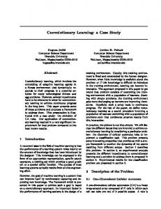
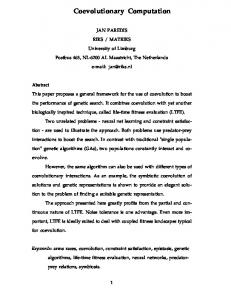
much, it is quite possible for the weaker player to win more games out n = 1000. If they were to play (say) n = 60, 000 games, then the two probability distributions overlap much less, as shown in Figure 2. p = 0.495 p = 0.505 0.025 0.02 0.015 0.01 0.005 0 440
460
480 500 520 Games won (out of 1,000)
540
560
Figure 1: For two strategies playing only n = 1000 games, the one that wins with probability p = 0.505 is barely discernible from its opponent who only wins with p = 0.495. 0.0035
Probability of winning that many games.
at playing the game. This means the co-evolutionary evaluation function escalates its level of difficulty, causing an “arms race” of ability. Numerous studies have followed this general approach on a variety of games and game-like tasks [22] [10] [13] [11] [16] [21]. Similar studies used two populations, where a member of one population is evaluated by how it performs against the members of the other population, and vica-versa [10].
p = 0.495 p = 0.505
0.003 0.0025 0.002 0.0015 0.001 0.0005
0 29200 29400 29600 29800 30000 30200 30400 30600 30800 Games won (out of 60,000)
Figure 2: For two strategies playing a massive n = 60000 games, the one that wins with probability p = 0.505 is more discernible from its opponent who only wins with p = 0.495.
2.1.2 The Binomial Distribution To find which of two players is better in a noisy game is nontrivial. Imagine a strategy that wins with probability p. The chances of it winning s successes out of n games is given by the binomial distribution [23, page 5]:
P (s wins out of n) =
n! ps (1 − p)(n−s) s!(n − s)!
(1)
Equation 1 gives a bell curve, whose spikiness increases as n increases. For example, consider two strategies of slightly different abilities: one wins with probability p = 0.505, the other with p = 0.495. If these were to play n = 1000 games, the distribution of wins is in Figure 1 — these overlap so
More games reduces the effect of noise, to detect small (but real) differences in ability. However, playing more games costs more computation time. 2.1.3 The Chance of Stupidity Winning Co-evolution is misled when a worse strategy beats a more capable strategy. How likely is that? For a player that wins with probability p, the probability of it winning s or more games out of n is given by summing Equation 1 [23, page 6]:
P (No. of wins ≥ s) =
n X i=s
n! pi (1 − p)(n−i) i!(n − i)!
(2)
P (Mixup) =
n X
P (better wins s)P (worse’s wins ≥ s)
s=0
=
n X n!(pb )s (1 − pb )(n−s) s=0
s!(n − s)!
n X n!(pw )i (1 − pw )(n−i) i=s
i!(n − i)!
!
(3) Actually, Backgammon does not allow ties, so for any two strategies pw = 1 − pb . But we are interested in a single strategy against every other member of the population, so we will keep the separate variable pw for clarity. For example, imagine a population of 100 players, where: • a single strategy can beat the other 99 with probability 0.505 • thus, the other 99 win with only 0.495 probability against that single better player • the single better strategy wins against itself with probability 0.5 • and those other 99 win against each other with probability 0.5 In this example, each of those 99 clones can expect to win with pw = 0.49995 of all the games, while the single better player can expect to win with pb = 0.50495. So we abuse notation and say things like pw = 0.5 and pb = 0.505 as a close approximation, but there are still no ties in Backgammon. The number of games n should be large enough to reduce Equation 3’s chance of a mixup to a rare event. Using Equation 3, Figure 3 shows the chance of a superior strategy doing no better than a worse rival (where 0.501 ≤ pb ≤ 0.505 and pw = 0.5) for various values of n the number of games. That is, Figure 3 tells us how often luck beats skill — as the real difference in ability shrinks, more games are needed. 2.1.4 The Effect of Noise on a Co-Evolving Population Imagine a thousand coins, one of which comes down heads 50.5% of the time, while all the others are fair coins. Toss each coin ten times. There is a 1-in-1024 chance of a fair coin coming up heads ten times out of ten, so one of the fair coins should get ten heads out of ten, and a bunch more should get nine. The biased coin can expect to get merely 5.05 heads out of ten. So — ironically — the biased coin (with its small but real difference) is almost certainly not going to come up heads the most, making it difficult to detect among the luckiest few of the unbiased coins1 . The larger the population, the more
Chance of a p=50% strategy winning more
How many games are necessary to detect the better of two strategies with almost the same ability? Putting together Equations 1 and 2, Equation 3 gives the chance of a mixup, i.e., where the better strategy (with p = pb ) does no better than its worse rival (with p = pw , where pb > pw ).
0.5 0.45 p = 0.501
0.4 0.35 0.3
p = 0.502
0.25 0.2
p = 0.503
0.15
p = 0.504
p = 0.501 p = 0.502 p = 0.503 p = 0.504 p = 0.505
0.1 0.05
p = 0.505
0 0
10000
20000 30000 40000 n = Number of games
50000
60000
Figure 3: For a strategy whose probability of winning a game pb is slightly greater than 0.5, this shows the chances the probability of such a superior strategy actually winning fewer games (out of n games, for various values of n) than an opponent (or population of opponents) winning with probability pw = 0.5. the effects of luck swamp the effects of skill. Figure 3 demonstrates that when the real differences in ability are small, it becomes unlikely that slightly-better individuals will be detected. More games are required, not merely to compare one strategy with another, but to compare one strategy with the luckiest few of a large population. This increases the necessary computation time. But just how many games are necessary? Do we need to detect a strategy that wins with probability 55%, or 51%, or 50.00001%? To answer this question, a co-evolutionary genetic algorithm learns to play the game of Backgammon in Section 3.
3 Co-Evolutionary Learning of Backgammon Genetic drift tends to make an evolving population converge to near-identical copies of each other. In such a population, Figure 3 suggests that the smaller the differences in ability, the more computation is necessary to detect that difference and thus avoid stagnation and continue learning. The Devil’s Advocate argument is that further learning is strictly proportional to more computation time. If this were so, it makes the whole approach very expensive in CPU time. This section describes a typical co-evolutionary learning system. Section 4 demonstrates the effects the amount of computation has on learning performance. 3.1 Experimental Setup 3.1.1 Backgammon and a Benchmark
1 Something
similar is accused of happening among mutual fund managers [7], now that there are thousands of mutual funds: if fund managers behave in a purely random manner, then a few would nonetheless enjoy outstanding returns, just as one coin in a thousand will come down ten heads in a row.
The game of Backgammon makes a suitable learning task. It uses dice, so there is a strong element of random noise — an expert will occasionally lose to a novice’s lucky dice rolls.
To measure the performance of the strategies produced by co-evolution after it has finished learning, we need some fixed, outside opponent to permit an off-line comparison (but co-evolution does not learn against an outside expert). Backgammon is popular, so many computer players are available as benchmarks. For a benchmark, we use the Backgammon strategy Pubeval, courtesy of Gerald Tesauro. Pubeval uses a very simple representation. To allow a fair comparison with this player, the co-evolutionary system also uses Pubeval’s simple representation, as described in Section 3.1.2. 3.1.2 A Strategy’s Architecture To allow a comparison with the benchmark Pubeval, each individual in the co-evolving population has the same architecture as Pubeval. Pubeval (and each strategy in the population) is a move evaluation function. Each move, a pair of pseudorandom dice are rolled, and a legal move generator produces the board position of every move that can be reached from the current board with those dice rolls. The move evaluation function returns a value for each of those possible board positions. The one with the highest value is taken. Pubeval uses an extremely simple neural network, merely a linear function — there are no hidden nodes nor extra layers. Actually, Pubeval is two linear functions, one for the main part of a game of Backgammon, the other for the final “racing” stage, when pieces do not have to pass opponent’s pieces. There is an algorithm for choosing the optimal move during the final, racing, stage of the game. Therefore, coevolution here only optimizes the first linear function, which evaluates moves during the main part of the game. The move evaluator for the racing part of the game is kept constant at the same values that Pubeval uses. The move evaluator has 122 inputs: • one to indicate how many of one’s own pieces are on the bar. • one to indicate how many of one’s own pieces are off the board. • For each of the board’s 24 positions, 5 inputs: • One if this position is occupied by only one of the opponent’s pieces2 • Four more, for counting one’s own pieces. The output is the sum of the products of the input and its corresponding weight: no sigmoid function nor hidden nodes. Co-evolution merely manipulates the values of the 122 weights — there is no backpropagation. A more elaborate architecture, with sophisticated feature detectors, would no doubt have evolved a better Backgammon player. However, this paper uses Backgammon merely as a typical noisy task, with many features of real-world problems, rather than because of any specific interest in that game. 2 In Backgammon, one can move to a board position occupied by only one opposing piece, but not to a position occupied by more than one opposing piece. Since it is not a legal move, there is no detector for multiple opposing pieces.
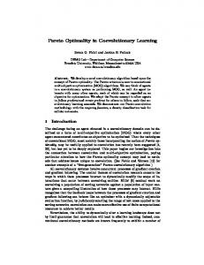
3.1.3 Fitness Function and Other Parameters A strategy’s fitness is the number of games won by playing all the members of the current population (including itself) for a fixed number of games per pairwise interaction. That fixed number is as low as 10 games for some runs, and as high as 100. For example, a run in Figure 4 has a population of 100 playing all-against-all, giving 5050 pairwise interactions. At 10 games per pairwise interaction, each generation requires just over fifty thousand games. At 100 games, over half a million games are played each generation. Other details of the implementation are as follows: • Population size is either 100 or 200. • Each of the 122 weights are represented as real numbers, not bit strings. • Elitism of 5%, that is, the best 5% of the population are copied without change. • Linear ranked fitness; the best individual expects 2 offspring, the worst expects none. • Uniform crossover. • Each allele has a 10% chance of being mutated, if it’s not crossed over. • Gaussian mutation: mean 0, standard deviation 0.05. • Initial values are uniformly random between -7 and +7, covering Pubeval’s values. We used the PGA-Pack software package3 and the MPICH implementation4 of the Message Passing Interface for parallel machines [9]. Even on parallel hardware, each GA run takes days to complete, so we have not yet accumulated enough runs for statistical significance testing. But the results presented below are representative, and we are confident that extra runs will bring no surprises. 3.2 Measuring Genetic Diversity A popular measure of genetic diversity is the Shannon index 5 : given n different groups, each of which has fraction fi of the total number of individuals, the Shannon index is [24]: H=
n X
−fi ln(fi )
(4)
i=1
A population of Backgammon strategies has no clearly partitioned groups. However, for any given board position, the population partitions itself according to what move they want to make next. So on a per-move basis, the population’s diversity can be measured with Equation 4. A single board position would not give a fair measure of diversity — what if the whole population agreed on what to 3 Available at http://www.mcs.anl.gov/˜levine/PGAPACK courtesy of David Levine of the Argonne National Laboratory. 4 Available at http://www.mcs.anl.gov/mpi, courtesy of the Argonne National Laboratory and Mississippi State University. 5 Also known as any of the Shannon-Weaver index, Shannon-Wiener index, or Shannon-Weaver-Wiener index.
do for that particular board position? To provide a representative sample, we generated 1306 board positions by playing Pubeval against itself for 20 games. Measuring the Shannon index of a population for each of these 1306 board positions, gives the mean and the standard deviation of the mean. This measure of diversity is used in Section 4.4 and Figure 6. This method of measuring diversity is imperfect, because it does not directly measure the difference in ability of strategies in the population. However, it suffices because it is consistent; we only need a way to compare two populations’ diversity relative to each other, and not with any absolute standard.
neat stratification. The run with only 10 games per interaction is ahead of the run with 30 games, at least for a while. If more games automatically gave better learning (as the Devil’s Advocate argument holds), then this wouldn’t happen. This anomaly is explained in Section 4.4.1. 4.2 Results: Population 200 Figure 5 shows two typical runs with a population of 200. Its most significant feature is that it does not display the neat stratification of Figure 4 at generation 500. In fact, using 50 games instead of 10 per interaction brings no improvement at all. 0.52
4 Results and Discussion Co-evolution does not learn from some fixed, external strategy. However, a convenient way to measure the performance of co-evolutionary learning is to compare the finished results to an unseen benchmark opponent. As described in Section 3.1.1, we use Gerald Tesauro’s Pubeval as the benchmark strategy. For various runs of a population of 100, Figure 4 shows the average performance against Pubeval — each member of the population plays 100 games against Pubeval. Winning 50% would indicate parity.
0.48 0.46 For population 200: 10 games per evaluation 50 games per evaluation
0.44 0.42 0.4 0.38 0.36 0.34 50
100
150
200 Generation
250
300
350
Figure 5: This shows the population’s average performance against the benchmark strategy Pubeval. For a population of 200, there is enough variation that extra sampling is unnecessary.
0.5
Pop. avg. wins against Pubeval
Pop avg wins against Pubeval
0.5
4.1 Results: Population 100
0.45 0.4 0.35 For population 100: 10 games per pairwise evaluation 30 games per pairwise evaluation 100 games per pairwise evaluation
0.3 0.25 0.2 0.15 0.1 0
100
200
300 400 Generation
500
600
Figure 4: This shows the population’s average performance against the benchmark strategy Pubeval. For the same population size of 100, all plays against all for a fixed number of games per pairwise interaction. The most interesting feature of Figure 4 is that even though learning stagnates by around generation 500, it stagnates at a higher ability given more games. There is a neat stratification around generation 500: the more games per pairwise evaluation, the more it wins against Pubeval. This would appear to agree with the argument that noise is bad for coevolution — more games are needed to discern finer differences and avoid stagnation. However, in Figure 4 around generation 100, there is no
More games do not necessarily give better learning: here, they’re redundant. This demonstrates that, although the number of games has some effect in Figure 4, more games give no advantage in Figure 5. Population size is the variable that dominates. This rebuts the gloomy Devil’s Advocate argument that co-evolution’s performance depends only on computation time. Also, the runs in Figure 5 perform better against the benchmark Pubeval than the runs in Figure 4. i.e., the larger population learns more. In fact, they average more than 50% against Pubeval, indicating a slight advantage, even with the same architecture as Pubeval. Thirdly and most surprisingly, the larger populations are faster. Not only do they take fewer generations — learning peaks around generation 300 in Figure 5 instead of generation 500 in Figure 4 — but each generation is faster: • The best run in Figure 4, with a population of 100 has 5050 pairwise interactions, which at 100 games per interaction uses more than a half-million games per generation. It tops out at less than 50% against Pubeval. • The quicker run in Figure 5, with a population of 200 has 20100 pairwise interactions. At only 10 games
per interaction, it takes just over two hundred thousand games per generation. This is only 40% of the best run in Figure 4, and nonetheless it tops out at more than 50% against Pubeval. So, in contrast to the gloomy argument that coevolutionary learning depends only on more CPU time, we find that a large enough population learns more from less computation. 4.3 Inconsistencies In Devil’s Advocate Argument So why is it that, with less computation and fewer games, Figure 5 learns better and faster than Figure 4, and beats Pubeval? This is completely inconsistent with the argument that more games are necessary for more learning. Even within Figure 5, playing more games per interaction (50 instead of 10) brings absolutely no advantage — it learns no faster, and tops out no higher. And even with the smaller population, the neat stratification at the end of Figure 4 is not present earlier on: the run with only 10 games per pairwise interaction is ahead of the run with 30 games, until about generation 250. This anomaly is explained in Section 4.4.1. 4.4 Large Population Maintains Diversity Using the measure of genetic diversity described in Section 3.2, Figure 6 shows the diversity of the runs shown in Figures 4 and 5. A population of 100 is, apparently, too small for this learning task and converges prematurely. Having done so, only a grinding comparison of the few small differences in the population can cause further improvement.
Avg Shannon index (diversity)
0.18
Population 100, 10 games Population 100, 30 games Population 100, 100 games Population 200, 10 games Population 200, 50 games
0.16 0.14 0.12 0.1 0.08 0.06
4.4.1 Benefits of Fewer Games Interestingly, of the two runs that use a population of 200 in Figure 6, the one that plays fewer games is more diverse. This is presumably because early in the run, when a small number of individuals are better than their near-random peers, fewer games help some of those near-random peers survive longer and thus pass their few useful traits on. Instead of a few “super individuals” dominating, some of the others get a chance, and this enhances diversity. Similarly, Figure 6 also explains the anomaly in Figure 4: why does the run with only 10 games per pairwise interaction learn faster (for a while) than the run with 30 games? • From Figure 6, until generation 250 the run with 10 games has more diversity than the run with 30. • From Figure 4, until generation 250 the run with 10 games learns faster than the run with 30. Again, the run with only 10 games per interaction means that a few “super individuals” do not entirely dominate, allowing some lucky but mediocre strategies to survive long enough to increase diversity. But because the population is too small, this eventually collapses into premature convergence: after about generation 250, its diversity in Figure 6 is no more than the other runs with population 100. Having fewer games actually enhances diversity, even early in a run which later converges prematurely. So long as it’s still sufficiently many games to discern the differences that exist, more games do not improve learning — they slow learning down, and run the risk of actually causing premature convergence by reducing diversity. Of course, even with the larger population, one can have too few games. We found that less than 10 games per pairwise interaction would reduce the final Backgammon ability. What is surprising is that more than 10 games (even a whopping 50 games per pairwise interaction, a million games per generation, as in Figure 5) did not improve ability, in stark contrast to Figure 4. There seems to be an optimal level of uncertainty here. This resembles simulated annealing, where some imprecision is a good thing — too much or not enough imprecision at the wrong time is bad for learning. Even with hill-climbing [20], it is conjectured that some noise is beneficial.
0.04
4.5 Relationship to Previous Work
0.02 50
100
150
200
250 300 Generation
350
400
450
500
Figure 6: This shows the genetic diversity of each run. Larger populations maintain more diversity. With enough variation, fewer games are needed to discern differences in ability. The runs with population 100 do not have error bars, for clarity. In contrast, a population of 200 maintains so much diversity that relatively few games are necessary to discern differences, and learning keeps going. In fact, it does so at lower computational cost than the smaller population.
Some previous studies have looked at imprecise evaluation in evolutionary computation. One study [19] did follow an approach where each individual’s fitness was based on a fixed number of encounters in a co-evolutionary context. Another study [4] looked more closely at the tradeoffs between (1) the amount of effort spent on evaluating each structure, and (2) the number of structures evaluated during a given generation. Theoretical analysis showed that, in some cases, more efficient search results from less accurate evaluations. However, this study goes a step further. With enough diversity in a larger population, more can be learned with less
computation than with a smaller population that cannot maintain enough diversity. Furthermore, even with a population large enough to maintain sufficient diversity, massive increases in CPU time do not find a better solution, as evinced by Figure 5.
the number of evaluations. However, the level of noise in Backgammon is fixed by the rules of the game — you can’t throw the dice any more or less often. A study that varies noise would have to use a different learning task.
5 Conclusion 4.6 Future Research 4.6.1 Implementation The scheme used here is a basic approach, because our focus is not about Backgammon as such, but about co-evolutionary learning on noisy tasks. Nonetheless, the question of how to make create better Backgammon player is one that is often asked — especially since Gerald Tesauro [25] used a machine learning method to create a Backgammon player (named TDGammon) comparable to the world’s best human players. The most obvious change is to strategy representation. Here, and in Pubeval, a strategy is a simple linear function for evaluation moves with only 122 weights. Tesauro’s TDGammon uses a conventional feed-forward network, with (in its current version) 160 hidden nodes, and thus thousands of weights. This would increase the necessary CPU time for coevolution. To reduce the computational cost, some innovations suggest themselves. Here, the number of games played by the population is fixed at a constant value for the whole of the run. Since few games are needed early in a run (both to discern the larger differences that exist, and to promote diversity by not being too harsh on the poorer performers), the number of runs could gradually increase during the run. This is a way to reduce computation time. Also, since playing more games (beyond a certain point) does not bring any improvement in Figure 5, there is no point in playing more games than that minimum. For a large population, if all play against all then it might turn out to be more than necessary. If so, it not all-against-all, but only allagainst-some may be enough games to discern differences in ability. This can also reduce computation time.
It could be argued that co-evolutionary learning might be unsuited for noisy tasks: genetic drift tends to produce a population of similar individuals, whose increasingly fine differences in ability need more and more evaluations to discern. A large population size could exacerbate this effect, because a slightly-better individual is not merely competing against one opponent, but against the luckiest few opponents in the entire population. However, this argument is incomplete. In a population large enough to avoid premature convergence, its diversity is enough for a modest number of evaluations to discern differences. In fact, with a large enough population, more evaluations than necessary fails to improve learning. Surprisingly, a larger and more diverse population allows better learning from less computation, than from a smaller population — a free lunch. On noisy tasks, the effect of population size, and thus diversity, dominates the effect of more sampling. Therefore, for many practical applications which suffer from random noise, co-evolutionary learning is feasible.
Acknowledgments The authors are grateful for discussions with members of Brandeis University’s DEMO Lab, and members of the University of Queensland’s Cognitive Science Group. We used PGA-Pack software and the MPICH implementation of the Message Passing Interface for parallel machines, courtesy of the Argonne National Laboratory and Mississippi State University. We are grateful to Gerald Tesauro for making Pubeval’s weights available. Paul Darwen’s research is partly supported by the Australia Research Council. Jordan Pollack’s research is partly supported by the Naval Research Laboratory and the National Science Foundation.
4.6.2 Other Tasks TD-Gammon’s representation does not only use the raw board positions as inputs — some inputs are certain features known to be useful for a Backgammon player, requiring human-constructed feature detectors. To know what features are useful to play Backgammon requires a priori expertise in the game. This is by no means an obstacle, but it increases the human engineering effort, and gets away from one of the strengths of evolutionary computation — that it can make progress on tasks with little prior knowledge. Better to take what we have learned here on Backgammon, and apply it to a different problem. It would be interesting to vary the level of noise, as opposed to keeping noise at a constant level while varying
Bibliography [1] Robert M. Axelrod, “The evolution of strategies in the iterated prisoner’s dilemma”, in Genetic Algorithms and Simulated Annealing, Lawrence Davis, Ed., chapter 3, pp. 32–41. Morgan Kaufmann, 1987. [2] David M. Chess, “Simulating the evolution of behavior: the iterated prisoners’ dilemma problem”, Complex Systems, vol. 2, pp. 663–670, 1988. [3] Paul J. Darwen and Xin Yao, “Speciation as automatic categorical modularization”, IEEE Transactions on Evolutionary Computation, vol. 1, no. 2, pp. 101– 108, July 1997.
[4] J. Michael Fitzpatrick and John J. Grefenstette, “Genetic algorithms in noisy environments”, Machine Learning, vol. 3, no. 2/3, pp. 101–120, 1988. [5] David B. Fogel, “Evolving behaviours in the iterated prisoner’s dilemma”, Evolutionary Computation, vol. 1, no. 1, pp. 77–97, 1993. [6] Richard P. Gagan, “Artificial intelligence in training applications”, Electronic Progress, vol. 21, no. 1, pp. 22– 27, 1992. [7] David Gardner and Tom Gardner, The Motley Fool Investment Guide, Fireside, 1997. [8] David E. Goldberg, Kalyanmoy Deb, and James H. Clark, “Genetic algorithms, noise, and the sizing of populations”, Complex Systems, vol. 6, pp. 333–362, 1992. [9] W. Gropp, E. Lusk, N. Doss, and A. Skjellum, “A highperformance, portable implementation of the MPI message passing interface standard”, Parallel Computing, vol. 22, no. 6, pp. 789–828, Sept. 1996. [10] W. Daniel Hillis, “Co-evolving parasites improve simulated evolution as an optimization procedure”, in Artificial Life 2, Christopher G. Langton, Charles Taylor, J. Doyne Farmer, and Steen Rasmussen, Eds., vol. 10 of Santa Fe Institute Studies in the Sciences of Complexity, pp. 313–323. Addison-Wesley, 1991. [11] Philip Husbands and Frank Mill, “Simulated coevolution as the mechanism for emergent planning and scheduling”, in Proceedings of the Fourth International Conference on Genetic Algorithms, Richard K. Belew and Lashon B. Booker, Eds., pp. 264–270, Morgan Kaufmann, 1991. [12] Takashi Ikegami, “From genetic evolution to emergence of game strategies”, Physica D, vol. 75, pp. 310–327, 1994. [13] Hugues Juill´e and Jordan B. Pollack, “Co-evolving intertwined spirals”, in Proceedings of the Fifth Annual Conference on Evolutionary Programming, pp. 461– 468, 1996. [14] Wei-Po Lee, John Hallam and Henrik H. Lund “A hybrid GP/GA approach to co-evolving controllers and robot bodies to achieve fitness-specific tasks”, in Proceedings of the 1996 IEEE Conference on Evolutionary Computation, pp. 384-389, IEEE Press, 1996. [15] Kristian Lindgren, “Evolutionary phenomena in simple dynamics”, in Artificial Life 2, Christopher G. Langton, Charles Taylor, J. Doyne Farmer, and Steen Rasmussen, Eds., vol. 10 of Santa Fe Institute Studies in the Sciences of Complexity, pp. 295–312. Addison-Wesley, 1991.
[16] David Moriarty and Risto Miikkulainen, “Discovering complex Othello strategies through evolutionary neural networks”, Connection Science, vol. 7, no. 3, pp. 195– 209, 1995. [17] Christian Nottola, Fr´ed´eric Leroy, and Franck Davalo, “Dynamics of artificial markets: Speculative markets and emerging “common sense’ knowledge”, in Proceedings of the First European Conference on Artificial Life, 1992, pp. 185–194, MIT Press. [18] Rorbert G. Palmer, W. Brian Arthur, John H. Holland, Blake LeBaron, and Paul Tayler, “Artificial economic life: a simple model of a stockmarket”, Physica D, vol. 75, pp. 264–274, 1994. [19] Jan Paredis, “Coevolutionary constraint satisfaction”, in Proceedings of the Third Conference on Parallel Problem Solving from Nature, Yuval Davidor, HansPaul Schwefel, and Richard M¨anner, Eds. 1994, vol. 866 of Lecture Notes in Computer Science, pp. 46–55, Springer-Verlag. [20] Jordan B. Pollack and Alan D. Blair, “Co-evolution in the successful learning of Backgammon strategy”, Machine Learning, vol. 32, no. 3, pp. 225–240, 1998. [21] Mitchell A. Potter, Kenneth A. De Jong, and John J. Grefenstette, “A coevolutionary approach to learning sequential decision rules”, in Proceedings of the Sixth International Conference on Genetic Algorithms, Larry J. Eshelman, Ed., pp. 366–372. Morgan Kaufmann, 1995. [22] Christopher D. Rosin and Richard K. Belew, “Methods for competitive co-evolution: Finding opponents worth beating”, in Proceedings of the Sixth International Conference on Genetic Algorithms, Larry J. Eshelman, Ed., pp. 373–380. Morgan Kaufmann, 1995. [23] Steven L. Salzberg, “On comparing classifiers: Pitfalls to avoid and a recommended approach”, Data Mining and Knowledge Discovery, vol. 1, no. 3, pp. 317–327, 1997. [24] Claude E. Shannon and Warren Weaver, Mathematical Theory of Communication, University of Illinois Press, Urbana, Illinois, 1949. [25] Gerald Tesauro, “Practical issues in temporal difference learning”, Machine Learning, vol. 8, pp. 257–277, 1992. [26] Xin Yao and Paul J. Darwen, “An experimental study of N-person iterated prisoner’s dilemma games”, Informatica, vol. 18, pp. 435–450, 1994.