Coevolutionary Computation JAN PAREDIS RIKS / MATRIKS University of Limburg Postbus 463, NL-6200 AL Maastricht, The Netherlands e-mail:
[email protected]
Abstract This paper proposes a general framework for the use of coevolution to boost the performance of genetic search. It combines coevolution with yet another biologically inspired technique, called life-time fitness evaluation (LTFE). Two unrelated problems - neural net learning and constraint satisfaction - are used to illustrate the approach. Both problems use predator-prey interactions to boost the search. In contrast with traditional "single population" genetic algorithms (GAs), two populations constantly interact and coevolve. However, the same algorithm can also be used with different types of coevolutionary interactions. As an example, the symbiotic coevolution of solutions and genetic representations is shown to provide an elegant solution to the problem of finding a suitable genetic representation. The approach presented here greatly profits from the partial and continuous nature of LTFE. Noise tolerance is one advantage. Even more important, LTFE is ideally suited to deal with coupled fitness landscapes typical for coevolution.
Keywords: arms races, coevolution, constraint satisfaction, epistasis, genetic algorithms, life-time fitness evaluation, neural networks, predatorprey relations, symbiosis. 1
1. Introduction
In general, GAs are highly simplified and abstract computational models inspired by natural selection. The differences in "fitness calculation" in GAs and nature clearly illustrate this. Standard GAs apply an a priori defined fitness function (e.g. the function one wants to optimize) to an individual. They typically use an "all at once" calculation: individuals are evaluated immediately after their creation (i.e. birth). Fitness calculation in nature is substantially different. It consists of a continuous series of tests during an individual's life. Furthermore, these tests are not strictly pre-defined. They originate from a complex environment. This environment is not only influenced by the animal's own actions but also by the other individuals as well as other processes occurring in the world (e.g. climatological or geophysical changes). Summarizing one can say that - in contrast with GAs nature uses a far more partial but continuous fitness evaluation in order to adapt to a complex world. In nature, various feedback mechanisms between the individuals undergoing selection provide a strong driving force towards complexity. Predator-prey relations are the most well-known examples. There is a strong evolutionary pressure for prey to defend themselves better (e.g. by running quicker, growing bigger shields, better camouflage ...) in response to which future generations of predators develop better attacking strategies (e.g. stronger claws, better eye-sight ...). In such arms races, success on one side is felt by the other side as failure to which must be "responded" in order to maintain one's chances of survival. This, in turn, calls for a reaction of the other side. This process of coevolution can result in a stepwise increase in complexity of both predator and prey. As far as the author is aware of, Hillis [6] was the first to propose the computational use of predator-prey coevolution. Here, we will see that the
2
introduction of a partial, continuous fitness evaluation results in a robust, fine-grained, algorithm with a significantly increased performance. It also gives rise to a general coevolutionary framework able to address traditional problems in Computer Science and Artificial Intelligence. This new type of GA is called a Coevolutionary Genetic Algorithm (CGA). Two earlier applications based on predator-prey interactions illustrate the approach: the search for good classification neural networks and the search for solutions to constraint satisfaction problems. Earlier papers [10, 11] describe these applications in greater detail and compare the performance of a CGA with other GAs. Now, these applications are only used to illustrate the abstract CGA introduced here. Both examples use predator-prey relations to improve the power of artificial search. Obviously, many other mechanisms - not necessarily based on an inverse fitness interaction between members of the different species exist in nature. Symbiosis is such an important and widely occurring counterexample. It consists of a positive fitness feedback in which a success on one side improves the chances of survival of the other. As we will see, the same general framework can be used to exploit symbiotic interactions as well. The structure of this paper is as follows. The next section describes the general CGA. Section three and four briefly describe the two applications mentioned above. Section five describes the symbiotic CGA and evaluates its performance. Section six focuses on the robustness of the CGA. The seventh section explores the connections with other research. The paper closes with conclusions and avenues for future research.
3
2. The Coevolutionary Genetic Algorithm
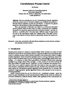
A large class of problems in Artificial Intelligence and Computer Science involve the search for a solution which meets certain a priori given criteria. The term "test-solution problems" is used here to refer to this class of problems. Inductive learning is an example of such a test-solution problem. It involves searching for an abstract concept description which generalizes given examples and excludes the given counterexamples. Constraint satisfaction is another example of the same type: one searches for a solution which satisfies the given constraints. In this section, we introduce the coevolutionary algorithm and illustrate it on the abstract class of "test-solution problems". Clearly, the search algorithm manipulates two types of elements: potential solutions (e.g. concept descriptions, potential solutions to a constraint satisfaction problem) and tests (e.g. examples, constraints). The basic population structures used by the CGA reflect this duality. In contrast with traditional single population GAs, CGAs operate on two interacting populations: one consists of potential solutions the other contains the tests. Figure 1 depicts the population structures used by a GA and a CGA.
a) SOLPOP
f i t n e s s e s
b) SOLPOP
f i t n e s s e s
Figure 1: Population structures used by a GA (a) and a CGA (b)
4
TESTPOP
f i t n e s s e s
A description of a traditional GA helps to introduce and characterize the main features of a CGA. Here, GENITOR [22,23] is used as an example of a traditional single population GA. It can be described as follows. First, the initial population of solutions is created. Furthermore, each solution has an associated fitness. For test-solution problems this fitness is the number of tests satisfied by the solution. Next, GENITOR repeats the following steps: 1) SELECT two parent solutions from the solution population. This selection is biased towards highly ranked individuals in the population which is sorted on fitness; 2) a new individual is generated from these parents through the application of MUTATION and CROSSOVER operators - in the examples described here we use adaptive mutation (see later) and the standard two-point crossover; 3) The FITNESS of the child is calculated by counting the number of tests it satisfies; 4) if this fitness is higher than the minimum fitness in the population then the child is INSERTed into the appropriate rank location in the solution population. At the same time, the individual with the minimum fitness is removed. In this way, the population remains sorted on fitness. The pseudo-code below describes the basic cycle of this "traditional single population" GA:
sol1:= SELECT(sol-pop) ; parent1 sol2:= SELECT(sol-pop) ; parent2 child:= MUTATE-CROSSOVER(sol1,sol2) f:= FITNESS(child) ; the number of tests satisfied INSERT(child,f,sol-pop)
The double population structure of a CGA now allows to extend the traditional GA in two ways. The first one is to replace the "all at once" fitness calculation of a GA with a more partial but continuous fitness evaluation which occurs during the entire life-time of an individual. This regime is called life-time fitness evaluation (LTFE). The second one is to allow both
5
populations to coevolve. Both extensions are described and motivated below. In a CGA, the set of all tests plays a much more prominent role than in the traditional GA described above. The fitness of a solution is now calculated on the basis of the tests it encounters (see later) during its life-time instead of on all tests at once. The fitness of a solution is defined as the number of tests satisfied by the solution during its last 20 encounters. Hence, each solution has a history which contains the results of its last 20 encounters with a test. Furthermore, the tests have a fitness as well. This fitness is defined as the number of times the test was violated by the 20 solutions it encountered most recently. Hence, the tests and solutions have an inverse fitness interaction, just as in predator-prey systems. The complete algorithm can now be described as follows. First, the solution and test populations are created. Typically, the members of the initial solution population are randomly generated. The tests, on the other hand, are known beforehand; they come with the problem specification. Hence, the initial test population typically contains these tests. In order to calculate the fitness of an initial solution, one counts the total number of satisfied tests out of twenty randomly chosen tests. Similarly, the fitness of a test is the number of solutions (out of a randomly chosen set of twenty solutions) which violate the test. Next, the following cycle is repeated. First, twenty solutions and tests are paired. During such an ENCOUNTER the solution is checked with respect to the test. The result of such an encounter is 1 if the test is satisfied or 0 in case of violation. This pay-off is pushed on the history of the solution involved in the encounter. At the same time, the pay-off of the least recent encounter is removed from the solution's history. Now, the fitness of a solution can be UPDATEd as well: it is set equal to the sum of the elements in its history. This corresponds to the number of satisfied tests. For the tests the inverse happens: they get zero pay-off when satisfied.
6
Otherwise, a 1 is pushed on the history. In both cases, the pay-off resulting from the oldest encounter in the history is removed. The fitness is, again, the sum of the pay-offs in the history. One should note that, just as in the traditional single population GA, the populations are kept sorted on fitness. As a consequence, an individual (test or solution) might move up or down in its population as a result of the update of its fitness. The continuous, partial fitness feedback resulting from the frequent execution of encounters is called life-time fitness evaluation (LTFE). It was first introduced in [10, 11]. After the execution of the encounters, the standard approach is followed: two solution-parents are SELECTed, a child is created and INSERTed in the solution population. Typically, the fitness of a "new-born" solution is initialized to the sum of the pay-offs obtained from 20 encounters with SELECTed tests. The code below describes the basic cycle of a CGA. The function TOGGLE in this basic cycle implements the inverse fitness interaction between tests and solutions. It changes a 1 into a 0 and vice versa.
DO 20 TIMES sol:= SELECT(sol-pop) test:= SELECT(test-pop) res:= ENCOUNTER(sol,test) UPDATE-HISTORY-AND-FITNESS(sol,res) UPDATE-HISTORY-AND-FITNESS(test,TOGGLE(res)) ENDDO sol1:= SELECT(sol-pop) ; parent1 sol2:= SELECT(sol-pop) ; parent2 child:= MUTATE-CROSSOVER(sol1,sol2) f:= FITNESS(child) INSERT(child,f,sol-pop)
In the code above, only the solution population truly evolves. This is because the test-solution problems addressed here require solutions to satisfy a fixed number of a priori given tests. In general one could, of course, evolve
7
both populations. In fact, this will be the case in an example discussed in a later section. Let us now look at the benefits gained from the use of LTFE. Its continuous partial nature allows for an early detection of good and bad solutions: the solutions do not need to be checked with respect to all tests. A few, well chosen, i.e. highly informative, tests provide sufficient information. This is true during different stages of the genetic search. In general, all solutions generated at the beginning of a run are rather bad. In this case, one does not need extensive testing. A rough indication of their quality is sufficient. Even if - due to an unlucky choice of tests in its initial encounters the fitness is rated a bit too low then future encounters will tend to raise this fitness. At later stages, LTFE is advantageous as well: it immediately weeds out clearly inferior offspring at minimal computational expense. When almost all solutions have a high fitness, e.g. they satisfy more than 80% of the tests, then clearly inferior solutions can be spotted quite easily. Here too, one does not need to check all tests. In a CGA, the fitness of the tests allows for a biased selection of tests as well. As a consequence, fit tests - i.e. tests not often satisfied by members of the solution population - are more often involved in an encounter. Or, in other words the algorithm focuses on the more difficult, not yet solved, tests. In this way, LTFE and the negative fitness interaction of the coevolution nicely complement each other. This will be demonstrated by the applications described in the following sections. In the code above, two additional parameters are introduced: the number of encounters before each reproduction and the number of most recent encounters used to calculate the fitness of the solutions and tests. In the code above and in all experiments in the rest of this paper, both parameters are set to 20.
8
3. Coevolutionary Neural Net Learning for Classification
This section illustrates the use of a CGA for classification on the task depicted in the left part of figure 2. Here, the CGA has to find appropriate connection weights such that a NN represents the correct mapping from [-1,1] × [1,1] to the set of classes {A, B, C, D} given 200 pre-classified, randomly selected, examples. This problem is designed such that the regions in the instance space ([-1,1] × [-1,1]) corresponding to the different classes have different degrees of complexity: class A consists of a circular convex region, class B is the union of two disjoint convex regions, C consists of one non-convex region, and D is the union of two non-convex regions.
1
B
D
A x
A
-1
1
y
B ....
C D
B
C -1
Figure 2: Left: Classification problem;
Right: Neural net classifier
The right part of figure 2 depicts the NN architecture used: a standard layered feed-forward network with one hidden layer consisting of 12 hidden nodes. As can be seen from figure 2, a correct neural net should classify, for example, the point (0.2,0.1) as belonging to class A. This classification pro9
ceeds as follows: 1) the coordinates 0.2 and 0.1 are clamped on the associated input nodes of the NN, 2) feed-forward propagation is executed - here the standard sigmoidal activation function is used, 3) the result of the classification is the class corresponding to the output node with the highest activity level. The NN is said to classify the example above correctly when the output node associated with class A is the most active one. Now, the traditional GA and the CGA can be applied on the classification task. Both algorithms encode the NNs as a linear string of their weights, with weights belonging to links feeding into the same node located next to each other. Both algorithms use a solution population of 100 NNs. The traditional GA tests each "new-born" NN on all 200 training examples at once. Hence, the fitness is defined as the number of training examples correctly classified by the NN. Table 1 describes the performance of the traditional GA on the classification task. It shows the number of offspring (in thousands) generated before a NN with a given level of classification accuracy (i.e.: 70%, 80%, 85%, 90%, and 95% of the 200 examples are correctly classified) is obtained. All experiments were repeated for 6 different crossover operators used during the reproduction of the NNs, i.e. in MUTATE-CROSSOVER. These crossovers - used in both algorithms (traditional and CGA) - were : one-point, two-point, four-point, six-point, twelve-point, and uniform crossover. Each crossover is followed by an adaptive mutation operator [23]. The probability of mutating a weight depends on the difference between the value of that weight in both parents. A difference larger than 0.01 results in a mutation rate of 0.001. For smaller differences, this probability increases linearly, reaching 0.02 when both parents have an identical weight value. Mutation replaces the weight in the offspring with a random value drawn from the interval [-100,100].
10
For each crossover 5 runs were executed. The best-so-far was averaged over these 5 runs. The traditional algorithm was allowed to generate a total of 50000 offspring. Table 1 shows, for example, that - on average - one-point crossover reaches a solution which correctly classifies 85% of the examples after generating 10500 offspring. Clearly, none of the crossover operators reaches an average best-so-far of 95% of correct classifications within the allowed 50000 offspring.
>70
>80
>85
>90
>95
1pt
2.5
8
10.5
17
-
2pt
2.5
5
7.5
13.5
-
4pt
3
8
10
-
-
6pt
3.5
5
11
21.5
-
12pt
4
7
10
22
-
uniform
6
10.5
14
20
-
Table 1: The traditional GA: empirical results. Each row gives the performance of the GA for one particular crossover. It shows the number of offspring (in 1000s) generated before a NN with a given level of accuracy is obtained. The data was obtained by averaging the best-sofar over 5 runs of 50000 cycles.
Table 2 shows the performance of the CGA. In addition to the solution population, the CGA has a test population. Here, this population contains the 200 pre-classified training examples. During an ENCOUNTER the NN classifies the example it is paired up with. The result of such an encounter is 1 if this classification is correct or 0 if incorrect. As was discussed in section 2, the basic cycle of the CGA consists of 20 encounters followed by the generation of one NN. Due to the partial nature of LTFE, the execution of the basic cycle of the CGA is 3.75 times faster than that of the traditional algorithm. The CGA was allowed to generate 100000 offspring. Hence, it uses only a little bit more than half of the time allocated to the traditional algorithm.
11
>70
>80
>85
>90
>95
1pt
4
9
20
60
-
2pt
3.5
9.5
12
17
42.5
4pt
4
6.5
11
26
74
6pt
4
7.5
11
21.5
58
12pt
4
5.5
8
12.5
36.5
uniform
4.5
7
10
16
47.5
Table 2: The CGA: empirical results. Each row gives the performance of the GA for one particular crossover. It shows the number of offspring (in 1000s) generated before a NN with a given level of accuracy is obtained. The data was obtained by averaging the best-so-far over 5 runs of 100000 cycles.
The tables allow to compare both approaches along two dimensions: computational demand and solution quality. The former is measured by the number of offspring needed before attaining a given accuracy level. Because of the difference in execution time of their basic cycles, the computational demand of both algorithms is equal when the CGA requires 3.75 times more offspring than the traditional GA to reach a given accuracy level. The comparison of both table clearly shows that the CGA needs far less than triple the GA's number of offspring. This is even more outspoken at the higher levels of accuracy. At these levels, the CGA needs to generate roughly the same number of offspring as the traditional algorithm (except for one-point crossover). Four times out of six, it does not even need more offspring than the traditional algorithm to achieve 90% accuracy. Hence, the computational demand of the CGA is considerably smaller than that of the traditional GA. In addition to this, the CGA clearly beats the traditional algorithm in terms of solution quality. Despite its shorter running time, it attains higher levels of accuracy. Now, most of the experiments easily reach the 95% accuracy level! More detailed empirical comparisons - including the performance increase resulting from LTFE and coevolution separately - can be found in [10].
12
Basically, there are two reasons for the considerable performance increase. First, LTFE drastically reduces the amount of computing time spend on fitness evaluation. This because it allows for early detection of good and bad solutions. Once a NN is considered potentially good it is put under closer scrutiny. Second, coevolution forces the CGA to focus on not yet solved examples (because of the fitness proportional selection of the examples involved in an encounter). This last point can be easily observed in our classification task: after a while only the examples which are situated near the boundaries between different classes have a high fitness value and reside at the top of the population. This are indeed the points which are hardest to classify: the training examples in their neighbourhood belong to different classes. Figure 3 clearly shows this. The left part of this figure depicts the distribution of the 200 training examples over the instance space [-1,1] × [-1,1]. The right part, on the other hand, shows the twenty fittest (i.e. "most difficult") examples at an intermediate stage of the search.
Figure 3: Left: distribution of all 200 examples;
13
Right: distribution of 20 fittest examples
Summarising one can say that the combined use of LTFE and coevolution in CGAs leads to good solutions within a reasonable time. LTFE reduces the computation demand, coevolution increases the solution quality. These results are also confirmed in [13] which uses a CGA to find a neural network capable of controlling a bioreactor.
4. Coevolutionary Constraint Satisfaction
The investigation of efficient algorithms for solving combinatorial problems is an active area of research. This is because of the large number of "real-world" problems with a combinatorial nature. Consider, for example, the area of industrial planning - whether one looks at order acceptance, scheduling, line balancing, capacity planning or project planning - one is immediately confronted with their combinatorial nature. These problems all belong to the class of Constraint Satisfaction Problems (CSPs). CSPs typically consist of a set of n variables xi (i ≤ n) which have an associated domain, Di, of possible values. There is also a set C of constraints which describe relations between the values of the xi. (e.g. the value of x1 should be different from the value of x3 ). A valid solution consists of an assignment of values to the xi such that all constraints in C are satisfied. As an example of a CSP, consider the n-queens problem. It consists of placing n queens on a n× n chess board so that no two queens attack each other (i.e. they are not in the same row, column, or diagonal). A frequently used representation of this problem - which we use as well - consists of n variables xi. Each such variable represents one column on the chess board. The assignment x2=3, for example, indicates that a queen is positioned in the third row of the second column. Hence, the xi take a value from the domain {1,2, ...,n}. The constraints for this problem are simple:
14
• xi ≠ xj
i≠j
; row-constraint
• |xi - xj| ≠ |i-j|
i≠j
; diagonal-constraint
The first line above prohibits two queens to be placed in the same row. The second line ensures that no two queens are on a same diagonal. The column constraint (only one queen is allowed per column) is implicit in the representation. CSPs fit nicely in the CGA framework presented here. For the nqueens problem the solution population consists of n-dimensional vectors containing integers between 1 and n. The 2 × n constraints (n row-constraints and n diagonal-constraints) constitute the test-population. Again, there is an inverse fitness interaction. The solution receives a reward when it satisfies the constraint, it receives a penalty in case the constraint is violated. For the constraint involved in an encounter the result of an encounter is opposite: it gets a penalty when the solution encountered satisfies it and a reward in case of violation. Again, fit solutions and constraints are more likely to be involved in an encounter. Or in other words, good solutions have to prove themselves more often. At the same time, the algorithm concentrates on satisfying difficult, i.e. not yet solved, constraints. In the n-queen problem, for example, the diagonal-constraints rapidly move up in the population. This is because they check both diagonals. Hence, for every occupied board location, they constrain 2 × (n - 1) other locations. The row-constraints, on the other hand, only constrain the other n - 1 board locations in a row. The experiments were done with a 50-queens problem, i.e. n=50. Hence, there are 100 constraints. Both algorithms, TRAD and CGA, use a solution population with a size of 250. Mutation changes a component of a solution vector with an integer randomly drawn from the set {1,2,3 ..., 50}. Furthermore, two-point crossover is used.
15
Again, the CGA clearly outperforms the traditional GA. The CGA finds 7 out of 10 times a valid solution to the 50-queens problem. The standard GA finds no correct solution in 10 runs. Additional empirical results [11] show that it is the combination of LTFE and coevolution which boosts the power of a CGA. Either one of these mechanisms alone yields clearly inferior results. This conclusion is in total accordance with the findings obtained from the NN classification application described in the previous section. This application of a CGA also provides an interesting approach towards some well-known research issues of GAs. The first one involves problems with a high degree of epistasis. Such problems are typically hard to solve because the choices made during the search for a solution are closely coupled. In general, highly epistatic problems are characterized by the fact that no decomposition in independent subproblems is possible. In that case, it is difficult to combine solutions to subparts (through the manipulation of so called "building blocks") into a solution to the overall problem. This is bad news for genetic algorithms (GAs) which typically search by combining features of different "solutions". A small change to a solution of a highly epistatic problem might drastically change the quality of the solution. Holland [7] showed that for problems with a relatively low degree of epistasis, operators that splice together parts of two different individuals might yield good solutions. For such problems, sets of functionally dependent genes are relatively small. In that case, it becomes possible to use a string representation in which the "correlated" genes are placed near to each other. Once the GA finds good values for these genes, they are unlikely to be split apart during sexual reproduction. Hence, these good values will proliferate through the population. Analogously, independent genes should be located far apart from each other on the string. Otherwise there will be too little exploration: suboptimal values for these genes are unlikely to get dis-
16
rupted. This last case typically results in premature convergence. In general, a linear string might not be sufficient to place interacting bits near to each other, and to place non-interacting bits far apart. This is particularly the case when addressing problems with a high degree of epistasis, such as CSPs in which the constraints induce interactions between a large number of variables. In the CSP-CGA application described here, each constraint checks the consistency amongst a number of "genes" (here variables). Good values for such sets of correlated genes should then be combined in order to obtain a global solution. As is the case in other approaches, a traditional positional crossover tends to disrupt genes which are located far apart from each other. Fortunately, the constraints checking such "difficult genes" will rapidly become fit. In this way, more search effort will be devoted to these genes. This is particularly relevant for problems consisting of too many dependencies to be packed on a linear string. The n-queens problem used here is an example of this: each variable is related to each other variable. The uniformity of the constraints does not allow to say which variables are most tightly coupled. As a matter of fact, the degree of interaction between two variables is not constant over the search space. It strongly depends on the assignment of the other variables. LTFE together with coevolution enables a CGA to concentrate, at run-time, on the relevant difficult (sets of) genes. The CGA application presented here can be contrasted with other approaches which use penalty functions to take into account the degree of invalidity of a solution. The success of these approaches critically depends on the choice of a good penalty function [16]. Ideally, it should strike a balance between convergence towards suboptimal valid solutions (when the penalty function is too harsh) or towards invalid solutions (when too tolerant a penalty function is used).
17
The CGA gives rise to an "auto-adjusting" penalty function. This is because the fitness evaluation is a kind of a penalty function, i.e. it counts the number of constraint violations. The changing ranking of the constraints and the biased selection of constraints on which the solutions are tested, allows the CGA to focus on the more difficult - not yet satisfied - constraints. Or, in other words, the penalty function becomes more and more harsh as better solutions are found. Informally, one could say that the penalty function coevolves in step with the quality of the solution population. Schoenauer and Xanthakis [17] already observed that gradually adding constraints during the evolutionary search improves the results obtained. The CGA automatically performs such a gradual tightening of the problem by focusing on the not yet satisfied constraints. Over the last years, GAs have been extended to deal specifically with constrained optimization. Recently, Paredis [9] proposed GSSS, a general method for introducing domain knowledge - through the use of constraint programming - to guide the evolutionary search when solving constraint problems. Michalewicz and Janikow [8] define genetic operators designed to tackle problems involving numerical linear (in)equalities. Fortunately, a CGA can incorporate domain knowledge just in the same way as a GA. This is because the code of the traditional single population GA is an integral subpart of the code of CGA. Hence, all extensions to the genetic representation or operators of a GA can be incorporated in a CGA as well.
5. Symbiotic Coevolution with CGAs
This section investigates the symbiotic evolution of solutions and their genetic representations (i.e. the ordering of the genes). The discussion on building blocks in the previous section already stressed the importance of and difficulties with - the choice of a good genetic representation. That sec-
18
tion gave two factors which complicate this choice. Primo, one might not know the epistatic interactions in advance. As a matter of fact, weak search methods such as GAs, are typically used to attack problems about which little knowledge is available. Secundo, one linear ordering might not be sufficient to express all epistatic interactions. Both problems suggest to combine the search for a solution with the search for a good representation. The goal is not so much to find the optimal representation - which might not exist anyway. It is more important that the representation used at a particular moment reflects the state of the search process. Once a certain subproblem is solved then most of the individuals in the population have the correct values for the genes encoding this subproblem. These genes can then be put further apart again. Even if crossover disrupts these genes then they are unlikely to receive a different value from another individual. For this reason the representation used should reflect the state of the search process. If a certain subproblem is already solved then a reordering allows to concentrate on other subproblems and other epistatic linkages. Symbiotic coevolution offers a way to obtain such a tight interaction between solutions and representations. It consists of a positive fitness feedback in which a success on one side improves the chances of survival of the other. A representation adapted to the solutions currently in the population speeds up the search for even better solutions which in their turn might progress optimally when yet another representation is used. This section describes SYMBIOT, a symbiotic CGA which is tested on problems with varying degrees of epistasis. But first these test problems are described. A companion paper [12] investigates the performance of SYMBIOT on a well-known deceptive problem with a fixed degree of epistasis.
19
5.1. The Test Problems The class of test problems used here is taken from [4]. The goal is to solve the matrix equation Ax=b. The matrix A (dimension n by n) and the ndimensional vector b are given. The n-dimensional real-valued vector x has to be found. Or, equivalently, the following system of linear equations has to be solved: n
bi = ∑ aij x j
i = 1,...,n.
(1)
j =1
Except for the sign inversion, which allows to use the same "maximizationGA" throughout this paper, the fitness function is identical to the one reported in [4]: n n − ∑ ∑ aij x j − bi i =1 j =1
(2)
The diagonal elements of A are randomly chosen from the set {1,2,3,...,9 }. When all off-diagonal elements of A are zero then the problem is not epistatic, i.e. each component xi only contributes to its corresponding bi. By setting off-diagonal entries to non-zero, the degree of epistasis is increased: the more non-zero off-diagonal elements in A , the higher the degree of epistasis. Only if the elements on the diagonal (aii: i ∈ {1, ..., n}) and immediately above it (ai-1;i: i ∈ {2, ..., n}) are non-zero then the i-th equation couples xi and x i+ 1 . Due to transitivity, this means that all x-components are coupled. Hence, given an array with only non-zero diagonal elements one can gradually increase the degree of epistasis by setting elements immediately above the diagonal to non-zero. This procedure is used here in order to control the degree of epistasis.
20
In order to allow for easy experimentation, the bi are chosen such that all components xi of the solution to the system of equations are equal to 1. In all experiments reported here, n is equal to 10, i.e. A is a 10 by 10 matrix, and x and b both contain 10 components. For most instances belonging to the class of problems described above, the performance of a traditional single population GA critically depends on the representation used. Only in two extreme cases is the choice of representation irrelevant. The first one is when there is no epistasis, i.e. all non-diagonal elements of A are zero. In this case, different orderings of the xi on the string give - on average - the same performance. At the other extreme - with all elements immediately above the diagonal different from zero as well any representation will perform equally poorly. The main problem is that a traditional single population GA uses only one, a priori defined, representation. The next subsection describes how SYMBIOT gets around this problem.
5.2 SYMBIOT Just as every other CGA described here, SYMBIOT uses two coevolving populations. One population contains permutations (orderings), the other one consists of proposed solutions to the problem to be solved. Each member of the solution population is represented as a 10-dimensional vector containing real numbers. Each such vector uses the same a priori chosen representation. The n-th element of this representation represents the value of xn . As will become clear later, any other representation could have been used here. The main purpose of such a canonical representation is to allow for a uniform fitness calculation. The vectors of the initial solution population are filled with real numbers randomly drawn from the interval [-30,30]. A permutation is represented as a 10-dimensional vector which describes a re-ordering of solution genes. The permutation represented by the vector [5 7 8 ....], for example, reorders the genes of a solution such that the
21
fifth bit of a (canonical) solution comes in place one, the seventh bit in place two, etc. The permutation [10 9 8 7 6 ... 1], for example, reverses the ordering of the genes of a solution. The code below describes the basic cycle of SYMBIOT. One can immediately observe the strong resemblance with the code of the CGA given in section 2. As a matter of fact, SYMBIOT is a simple extension of that CGA. Now, the encounters involve two solutions and one permutation. First, the three individuals involved in an encounter are SELECTed from their respective population. Again, fitter individuals are more likely to be selected. Next, the selected permutation, perm, is applied to both solutions. The resulting gene-strings are then processed with standard (one-point) CROSSOVER and MUTATion in order to generate offspring. Hence, the permutation constructs the representation operated on by crossover. Finally, INVPERMUTATE applies perm - 1 to the child in order to reconvert it to the canonical representation such that its FITNESS can be calculated. Formula 2 of section 5.1 is used to calculate this fitness. The canonical representation of the child is then INSERTed in the population of solutions at its appropriate rank. Hence, each encounter results in the "birth" of a new solution. DO 20 TIMES sol1:= SELECT(sol-pop) sol2:= SELECT(sol-pop) perm:= SELECT(permut-pop) p-sol-child:= MUTATE-CROSSOVER(perm(sol1),perm(sol2)) sol-child:= INV-PERMUTATE(p-sol-child,perm) sol-f:= FITNESS(sol-child) INSERT(sol-child,sol-f,sol-pop) r:= ((FITNESS(sol1)+ FITNESS(sol2)) / 2) / sol-f UPDATE-HISTORY-AND-FITNESS (perm,r) ENDDO perm1:= SELECT(permut-pop) perm2:= SELECT(permut-pop) perm-child := ENHANCED-EDGE-RECOMB(perm1,perm2) perm-f := INIT-PERM-FITNESS(perm-child) INSERT(perm-child,perm-f,perm-pop)
22
As a next step, the fitness of a permutation needs to be defined. As in previous CGA applications, this fitness is the sum of the pay-offs received during the 20 most recent encounters the permutation is involved in. This fitness should give an indication of the quality of the permutation. As described above, a good permutation puts the relevant functionally correlated genes near each other. Unfortunately, SYMBIOT has no a priori knowledge about the epistatic interactions between the genes. It has to discover these correlations by itself. Only the (solution)fitness feedback can be used. Here, for every encounter, the permutation receives a pay-off equal to the average fitness of the parents divided by the fitness of the child1. A good permutation will - on average - generate good children. In this case, the pay-off - and hence also the fitness of the permutation - will be relatively large. Obviously, this measure is highly noisy and should be tested over a large number of encounters. Once again, LTFE takes care of this: during its lifetime each individual is frequently involved in an encounter. One difference with the two predator-prey CGA applications discussed above is that now only one population (the permutations) undergoes lifetime fitness evaluation. The solutions are rated - once and for all - immediately after their birth using formula 2. Another difference with the two predator-prey CGAs is that now, both populations really reproduce and evolve. Hence, the reproduction of the permutations remains to be discussed. One such a reproduction occurs after every 20 encounters. The most important information in a permutation is not the exact position of the genes or their relative order but the adjacency information: which genes are placed nearby each other. Hence, a "child permutation" should inherit such information from its parents. Starkweather et al [20] introduces "ENHANCED EDGE RECOMBination", a genetic operator designed specifically for this purpose. This operator is used here as well. 1 Remember that the fitness values of the solutions are negative.
23
In order to initialize the fitness of a permutation (INIT-PERMFITNESS), one encounter is executed between the permutation and two SELECTed solutions. All the elements in the history of the new-born permutation are initialized to the pay-off of this encounter. Again, a major advantage of LTFE is that permutations have to prove themselves all the time. In this way, LTFE averages out the noise in the fitness evaluation of a permutation. Mutation is one source of such noise. It may change the fitness of the child considerably (especially when dealing with highly epistatic problems) and hence also the pay-off received by the permutations. Fortunately, through the biased selection of individuals involved in an encounter, once a permutation is considered good, it has to prove itself more often. Moreover, LTFE allows the permutations to keep up with the changes in the solution population and vice versa. The next subsection introduces two traditional single population GAs. An empirical performance comparison of these algorithms and SYMBIOT allows us to get a better understanding of SYMBIOT's power.
5.3 FIXED and RAND: Two Single Population Algorithms. The first algorithm - called FIXED - is a traditional GA as described in section 2. It uses the best possible representation: a 10 dimensional vector x with the xi ordered on ascending index. Any other representation would give a lower performance, except at extreme low (or high) degrees of epistasis where all representations are bound to perform, on average, equally well (or poor). In contrast with SYMBIOT, FIXED has the advantage that it uses the best possible representation. SYMBIOT, on the other hand, still has to find a good representation. Or in other words, SYMBIOT not only has to solve the set of linear equations; it has to solve the representation problem as well. Hence, SYMBIOT can expect strong competition from FIXED. The experiments in
24
the next subsection allow to compare the performance of both algorithms on problems with different degrees of epistasis. A second "single-population" GA, called RAND, generates for each couple of parents, a RANDOM PERMutation which is applied before crossover and mutation. Next, INVERSE-PERMUTATion is applied to the child. In order to calculate its FITNESS and to INSERT it in the population at the appropriate rank. The code below describes RAND's basic cycle: sol1:= SELECT(sol-pop) sol2:= SELECT(sol-pop) perm:= RANDOM-PERM() p-sol-child:= MUTATE-CROSSOVER(perm(sol1),perm(sol2)) sol-child:= INV-PERMUTATE(p-sol-child,perm) sol-f:= FITNESS(sol-child) INSERT(sol-child,sol-f,sol-pop)
Unlike FIXED, RAND does not use the same a priori defined representation for each reproduction. The random ordering generated before each reproduction ensures that - on average - all genes have an equal probability of being transmitted together (i.e. coming from the same parent) to the child. The performance comparison of RAND and SYMBIOT in the next subsection allows to assess the value of SYMBIOT's evolutionary accumulation of good groupings of genes in the permutation population.
5.4 Empirical Results As mentioned above, SYMBIOT concurrently performs two searches: one for a good solution and one for a good permutation. Intuitively one would expect that this constitutes considerable overhead when solving problems without or with a low degree of epistasis. For high degrees of epistasis yet another problem might crop up: the fitness calculation of the permutations becomes less reliable. This is because small changes to solutions to highly epistatic problems might give rise to large changes in fitness. This is because, the fitness landscape of epistatic problems is rugged and uncorrelated. No 25
permutation can alleviate this problem: whatever the representation used, the correlation between the fitness of a child and its parents will remain low. That is why SYMBIOT is unfair when confronted with high degrees of epistasis: it blames the permutation when bad offspring are generated. The experiments described in this section allow to determine the degrees of epistasis at which SYMBIOT performs well. In all experiments, the size of the solution and permutation populations is 1000 and 100, respectively. Accordingly, the single population algorithms (RAND and FIXED) use a solution population size of 1000. All results are averaged over 10 runs. Two series of experiments are reported here. The first compares SYMBIOT with the single-population algorithms described above. This is done for problems with different degrees of epistasis. A second series of experiments shows the grouping of functionally related genes in SYMBIOT.
5.4.1 Performance comparison
Four different problems are used here. In
ascending degree of epistasis these problems are named: TRIVIAL, SIMPLE, MEDIUM, and COMPLEX. All use a matrix A with non-zero diagonal elements. They differ in the number of non-zero elements immediately above the diagonal. In all problems used here, all other elements of A are zero. TRIVIAL is a problem without any epistasis: all off-diagonal elements are zero. SIMPLE is slightly more epistatic, its variables are linked pairwise. These pairs are non-overlapping. Or more formally, the set of linkages is: {(x1,x2), (x3,x4), (x5,x6), (x7,x8), (x9,x10)}. These linkages are realized by setting the elements ai-1;i tot non-zero and this for all even i, i.e. a12 , a34 , a56 , a78 , a 9,10 are assigned values randomly drawn from the set {1,2,3,4,5,6,7,8,9}. The other two examples have still more linkages. The set of linkages of MEDIUM and COMPLEX are {(x1,x2), (x2,x 3), (x3,x4), (x4,x 5), (x5,x6), (x7,x8), (x9,x10)} , and {(x1,x2), (x2,x3), (x3,x4), (x4, x5), (x5,x6), (x6, x7), (x7,x8), (x8, x9), (x9,x10)}, respectively. Hence, in MEDIUM the variables x1,x2,x3,x4,x5,x 6 are
26
completely interlinked. In addition to this, x7 is linked with x8 and x9 with x10. In COMPLEX, each variable depends on each other variable. Hence, the series of problems used here gradually adds more epistatic links. The graphs in figure 4 show the evolution of the average fitness of the solution population over time and this for each of the four problems described above. Each graph has the same scale and size. This allows for easy comparison between them. The x-axis represents the number of solutions generated. It would be unfair to use the number of executions of the algorithm's basic cycle as x-axis. This is because SYMBIOT generates 21 solutions in one cycle (20 during the encounters and 1 to initialize the fitness of the new permutation). FIXED and RAND, on the other hand, only generate one solution per cycle. Several observations can be made from the data depicted in figure 4. Clearly, lower fitnesses are obtained when the degree of epistasis is increased. It also takes longer before the average fitness of the solution population becomes large enough to be depicted. The choice of representation should not influence the performance when solving the non-epistatic TRIVIAL problem. This is because of the independence of the TRIVIALgenes. Accordingly, the upper left graph in figure 4 shows that the three algorithms (RAND, FIXED, and SYMBIOT) have a comparable performance. When looking at SIMPLE, small differences start to appear. Both FIXED and SYMBIOT, perform equally well. RAND seems slightly worse. One would expect the good performance of FIXED. Its representation (the xis are placed in ascending order of i) is ideal for this problem: only strictly neighbouring genes interact. It looks as if SYMBIOT is able to keep up with FIXED, whereas RAND using random representations starts to have a more difficult time keeping up. This trend is much more pronounced in MEDIUM. Now, FIXED is unable to cater for the tight interactions between the first six variables. SYMBIOT now clearly outperforms FIXED. The performance of
27
Figure 4: Evolution of the Average Population Fitness for the Four Test Problems
28
RAND, on the other hand, is poor. In addition to this, the standard deviation of the performance of RAND (1.71) and FIXED (2.39) is considerably larger than that of SYMBIOT (0.28). Finally, we arrive at COMPLEX, the completely epistatic problem. Now all three algorithms perform rather poorly. The standard deviation of the performance data is now also considerably larger (FIXED: 4.91; RAND: 3.8; SYMBIOT: 2.85).
In
conclu-
sion, we can say that in comparison with RAND and FIXED, SYMBIOT is able to operate well over a larger range of degrees of epistasis. The results above also indicate that the symbiotic evolution helps SYMBIOT to focus on good representations. The experiments in the next subsection investigate this in greater detail. Obviously, for maximally epistatic problems the rugged and uncorrelated fitness landscape (of both solutions and permutations) provides too little information to guide the search.
5.4.2 SYMBIOT's grouping of related genes.
The second set of experiments
allows to assess the degree to which permutations group functionally related genes. First the term average defining length of a set of pairs of genes is introduced. The following step is central in its calculation: for a given permutation and a given pair of genes, one computes how far the permutation puts these genes apart. Or in other words, the distance between both genes is calculated. An example will certainly clarify this: consider a permutation which puts one gene at position 5 and the other one at position 8. The distance between these points is 3. The "average defining length of a set of pairs of genes" is the average of this distance for each pair of genes in the set and for each member of the permutation population. Hence, it measures the degree to which the permutations group the given pairs of genes together. For the 10-bit problem described above, this means that with a permutation population size of 100, 500 distances are averaged to compute the average defining length of a set containing 5 pairs of genes.
29
SIMPLE is the first problem used here. Remember SIMPLE's set of linkages: {(x1,x2), (x3,x4), (x5,x6), (x7,x8), (x9,x10)}. The curve labelled "related" in figure 5 depicts the evolution of the average defining lengths of this set of paired genes over time. The x-axis represents the number of solution offspring generated (in thousands). Again, the results are averaged over ten runs. One sees a steep drop of the average defining lengths. They drop from an initial 3.7 to just below 2.5. Or in other words, initially the related variables are - on average - a distance of 3.7 apart on the "gene-string". This average separation drops to a little bit less than 2.5. The curve labelled "unrelated" depicts the average defining lengths of the following pairs of unrelated variables: {(x2,x3), (x4,x5), (x6,x7), (x8,x9)}. One sees that this curve fluctuates around 3.7. The difference between both curves shows that SYMBIOT clearly exhibits a clear selective pressure towards grouping related variables and leaving unrelated genes apart.
AVERAGE DEFINING LENGTHS
4
UNRELATED 3.5
3
RELATED 2.5
2 0
50
100
150
200
#SOLUTION OFFSPRING (1000s)
Figure 5: Grouping of genes when solving "SIMPLE".
30
One point about figure 5 requires further explanation: why does the average defining length of the linked variables gradually increase after its initial drop? The reason for this is the following: during the search, the pairs of related variables are solved at different moments. Each time one such solution is found it becomes important to have permutations which group the variables involved. In this way, the good genetic material will spread quickly through the population. Or in other words, most individuals in the population will get these same values for these pairs of variables. Once, this has happened the probability of losing this genetic material through crossover is fairly low. Hence, there is not much selection pressure towards keeping these values together. Selection pressure will promote permutations which group the less frequently "solved" variables. At the later stages of a run, all solutions get more and more similar. As a result the selective pressure to group particular genes decreases. The same experiment was repeated on a problem with a higher degree of epistasis. This problem is called "5-5" because it consists of two sets of five variables. More exactly, 5-5 has the following set of linkages: {(x1 ,x 2 ), (x2,x3), (x3,x4), (x4,x5), (x6,x7), (x7,x8), (x8,x9) ,(x9,x10)}. This problem is only one linkage - (x5 ,x6 ) - away from total epistasis. The variables x1 ,x2 ,x3 ,x4 ,x5 are completely interlinked. The same is true for the other 5 variables. The curve in figure 6 labelled "related" now gives the average defining length of the shortest schema (substring) containing x1 ,x 2 ,x 3 ,x 4 ,x 5 and of the shortest schema containing x6 ,x 7 ,x 8 ,x 9 ,x 10 . If, for example, a permutation puts the variables at positions 8, 2, 4, 7 and 5, respectively then this defining length is equal to 6 (= 8 - 2). The curve "unrelated", on the other hand, averages these defining lengths for the variables x1 ,x 2 ,x 8 ,x 9 ,x 10 and x3 ,x 4 ,x 5 ,x 9 ,x 10 . Here again, the same trend can be seen: the "related"-curve quickly drops and then gradually increases again. The "unrelated"-curve, on the other hand, remains fairly stable at its initial value. This curve is less smooth than the
31
one given in figure 5. This is mainly due to the higher level of epistasis. As explained in subsection 5.4 the fitness evaluation of permutations becomes less reliable at higher degrees of epistasis.
AVERAGE DEFINING LENGTH
7.5
UNRELATED
7.4 7.3 7.2
RELATED
7.1 7 6.9 6.8 0
50
100
150
200
#SOLUTION OFFSPRING (1000s) Figure 6: Grouping of genes when solving "5-5".
The experiments described above show that SYMBIOT exhibits a distinct selective pressure towards grouping interacting genes together. One important point still remains to be made. In all experiments SYMBIOT used one-point crossover to recombine solutions. This operator has high positional bias, i.e. the probability that two genes are being inherited from the same parent is strongly - and positively - correlated with their proximity on the gene string. Operators with lower positional bias, such as two-point, or - even worse uniform crossover, negatively influence the performance of SYMBIOT. This is because a crossover with high positional bias will -with a large probability - leave together the genes grouped by a permutation. In other words, the relation between the fitness of the child and that of its parent is a good estimator of the goodness of the permutation. Consider at the other extreme what
32
happens when uniform crossover is used to create offspring. In this case, the fitness of the child is completely independent of the permutation applied to the parents before crossover. Hence, there will be no selective pressure on the permutations to group together related genes. The experiments described in [12] quantify the influence of the positional bias of the crossover used on the performance of SYMBIOT.
6. Steady-State Reproduction, Noise, and LTFE.
Syswerda [21] introduced the term steady-state reproduction for the one-at-atime reproduction used in systems like GENITOR. However, these systems are not very robust. They perform best on problems with a deterministic fitness evaluation function. Noisy fitness functions might pose serious problems to steady-state reproduction systems. Consider, for example, an individual which, due to noise, is assigned too high a fitness. In steady-state systems this fitness remains associated with that individual as long as it stays in the population. During all this time its overestimated genetic material may spread throughout the population. This problem does not occur when generational replacement is used. In that case, each generation creates an entirely new population and calculates the fitness of these members anew at each generation. Hence, an individual is re-evaluated each time it survives a generation. This way noisy evaluations do not substantially decrease the reliability of the sampling. LTFE does provide a good way to deal with noise within steady-state reproduction. This is due to the continuous fitness feedback which averages out the noise in the fitness evaluation. The symbiotic CGA application described here, clearly illustrates this. Currently, the author is setting up experiments to demonstrate and quantify this noise tolerance further. Hence, the research described here takes up the challenge described in Davis [2]:
33
Although no one has yet published a paper about steady-state reproduction with noisy evaluation functions, it seems possible that modifications to the steady-state algorithm can be devised that will outperform generational replacement on such problems. This is a fertile topic for future research.
7. Related Research
The work reported here differs from a lot of research in the field of Artificial Life, in that, it uses coevolution to solve well-known problems in Computer Science and Artificial Intelligence. Hence, coevolution does not emerge, it is built-in. Furthermore, CGAs are designed to solve "manmade" problems. They are not constructed to find adequate survival-behaviors in a simulated world. This same approach was also followed by Hillis [6], which provided the basic inspiration for the work presented here. He coevolved (using predator-prey interactions) sorting network architectures and sets of lists of numbers on which the sorting networks are tested. Through the introduction of LTFE, CGAs are more robust and fine-grained. This incorporation of LTFE is an important difference with Hillis' work. Moreover, we defined a large, abstract class of problems which can be solved with a CGA. In addition, the CGA can easily be extended to incorporate symbiotic interactions as well. Various links with research on genetic algorithms can be pointed out. The first one is the work on competitive fitness. Angeline and Pollack [1] describe competitive fitness as follows:
34
A competitive fitness function is any calculation for fitness that is dependent on the current population to any degree.
CGAs use a new type of competitive fitness function which differs in several aspects from previous approaches. First, a CGA operates on two populations containing different types of individuals (e.g. neural networks versus training examples or solutions to a CSP versus constraints). Second, there is the bias in the encounters and the continuous nature of LTFE. Hence, the pair-wise competition pattern used by CGAs could best be called: "biased continuous". The work described in [15] is relevant with respect to the symbiotic CGA. It introduces cooperative coevolutionary genetic algorithms (CCGAs). These algorithms have been tested in the domain of function optimization. This way, the natural decomposition into a fixed number of subcomponents (namely the parameters of the function to be optimized) can be exploited. Each population contains values for one parameter. The fitness of a particular value is an estimate of how well it "cooperates" with the other populations to produce a good overall solution. This involves global synchronous communication between the populations. The work on CCGAs and our work both use multiple interacting species to solve existing "man-made" problems. The basic mechanisms are, however, quite different (e.g. the identity of the individuals, the fitness calculation). Moreover, CGAs do not require (knowledge about) the decomposition of solutions. Finally, the particular application of a symbiotic CGA presented here addresses the well-known problem of finding good genetic representations. The use of an inversion operator - which randomly changes the ordering of the "genes" - is probably one of the oldest approaches to this problem. Unfortunately, it has proven rather unsuccessful. This is probably due to the random nature of the inversion operators. In contrast with inversion-based
35
genetic algorithms, SYMBIOT's reorderings are not random. They coevolve with the solutions. This has two advantages. Primo, it allows for the incremental construction of good permutations from other permutations. This way, SYMBIOT exploits the evolutionary accumulation of small improvements. Secundo, SYMBIOT finds permutations which reflect the state of the search process. Or in other words, it concentrates on "not yet solved" subproblems. This in contrast with more static approaches [19] which determine at the beginning of a run the representation to be used. Hence, SYMBIOT gets rid of the traditional fixed-coding approach. It does, however, stick to the usual fixed length coding. This in contrast with the messy GAs described in [5]. There is, however, a price to be paid when dropping the fixed length coding: fitness needs to be defined for all incomplete solutions as well. Through its fixed length coding, SYMBIOT does not rely on this assumption.
Conclusion and Future Research
This text introduces coevolutionary genetic algorithms. It combines a coevolutionary framework with life-time fitness evaluation. The partial and continuous nature of LTFE is ideally suited to deal with coupled fitness landscapes. Coevolutionary interacting species typically give rise to such coupled landscapes. The use of LTFE in combination with coevolution has several advantages: increased performance (this in terms of solution quality as well as computation demand) and noise tolerance. Interestingly, both the predator-prey CGA and the symbiotic CGA offer two different ways of dealing with problems with relatively high degrees of epistasis. The symbiotic approach is totally knowledge free. The predatorprey approach, on the other hand, uses domain knowledge (in the form of constraints).
36
Clearly, the CGA is inspired by coevolution as it occurs in nature. On the other hand, A CGA is used to solve "man-made" problems. As a result, the coevolution mechanism of a CGA differs in several ways from that in nature. A first difference is CGA's fixed population size of the coevolving populations. This excludes the possibility of a species going extinct. Also the notion of topology, i.e. the spatial distribution of individuals, is much simplified. Furthermore, problem characteristics might lead to various other differences with nature. In the predator-prey models for test-solution problems, for example, the tests do not evolve. The test population contains all the time the same tests. On the other hand, one could argue that LTFE is much closer to reality than the traditional "all at once" fitness calculation. Here also, problem characteristics might impose the type of fitness calculation to be used. In the case of SYMBIOT, for example, LTFE is used to rate the permutations. The solutions, however, are evaluated with an "all at once" fitness calculation. Different avenues for future research on CGAs are open for further exploration. First, CGAs can be applied to different problems and problem classes. This is the case for both classes of CGAs: predator-prey as well as symbiotic ones. Second, the usefulness of more complex coevolutionary interactions remains to be studied. Here one could, for example, think of more than two interacting populations in which symbiotic as well as predatorprey relations might possibly coexist. Two topics briefly mentioned in this paper need further investigation as well. One is the parallel implementation of a CGA. The fine-grained nature of a CGA allows for easy parallel implementation. A massively parallel architecture with each processor containing one solution and a (copy of) a test can be used. Efficient machine-level shift operations can change the partners involved in the encounters. Local selection and reproduction can then be implemented using the fine-grained parallel genetic algorithm de-
37
scribed in [18]. This point certainly warrants further research. Also the introduction of life-time learning and its integration with LTFE deserves further investigation. Results of initial experiments with this integration of learning within a CGA are reported in [14].
Acknowledgments This author would like to thank Melanie Mitchell for her comments and suggestions. The author is also indebted to Roos-Marie Bal and Séverine Dufour for proofreading this paper. This research was sponsored in part by the European Union as Brite/Euram Project No. BE-7686 (PSYCHO).
References [1] Angeline, P.J. & Pollack, J.B. (1993). Competitive environments evolve better solutions for complex tasks. In S. Forrest (Ed.), Proceedings of the Fifth International Conference on Genetic Algorithms (pp. 264-270). San Mateo, CA: Morgan Kaufmann. [2] Davis, L. (ed.) (1991). Handbook of Genetic Algorithms, New York: Van Nostrand Reinhold. [3] Eshelman, L.J., Caruana, R.A., & Schaffer, J.D. (1989). Biases in the crossover landscape. In J.D. Schaffer (Ed.), Proceedings of the Third International Conference on Genetic Algorithms (pp. 10-19). San Mateo, CA: Morgan Kaufmann. [4] Fogel, D.B., & Atmar, J.W., (1990). Comparing genetic operators with gaussian mutations in simulated evolutionary processes using linear systems, Journal of Biological Cybernetics, (pp. 111-114). Springer Verlag. [5] Goldberg, D.E., Korb, B., & Deb, K. (1989). Messy genetic algorithms: motivation, analysis , and first results, Complex Systems, 3 (pp. 493-529). [6] Hillis, W.D. (1992). Coevolving parasites improve simulated evolution as an optimization procedure. In Langton, C.G., Taylor, C., Farmer, J.D., & Rasmussen, S. (Eds), Artificial Life II (pp. 313-324). Redwood City, CA: Addison-Wesley. [7] Holland, J. (1975). Adaptation in Natural and Artificial Systems, Ann Arbor: Univ. of Michigan Press. [8] Michalewicz, Z., & Janikow, C.Z. (1991). Handling constraints in genetic algorithms. In R.K. Belew & L. B. Booker (Eds.), Proceedings of the Fourth International Conference on Genetic Algorithms (pp. 151-157). San Mateo, CA: Morgan Kaufmann. [9] Paredis, J. (1993). Genetic state-space search for constrained optimization problems. Proceedings of the Thirteenth International Joint Conference
38
on Artificial Intelligence (pp. 967-973). San Mateo, CA: Morgan Kaufmann. [10] Paredis, J. (1994). Steps towards coevolutionary classification neural networks. In R. Brooks, & P. Maes (Eds), Proceedings of the Fourth International Workshop on the Synthesis and Simulation of Living Systems (Artificial Life IV) (pp. 102-108). Cambridge, Mass: MIT Press/ Bradford Books. [11] Paredis, J. (1994). Coevolutionary constraint satisfaction. In Y. Davidor, H-P. Schwefel, & R. Manner (Eds.), Proceedings of the Third Conference on Parallel Problem Solving from Nature 2, Lecture Notes in Computer Science, vol. 866 (pp. 46-55). Berlin Heidelberg: Springer Verlag. [12] Paredis, J. (1995). The symbiotic evolution of solutions and their representations. In L. Eshelman (ed.), Proceedings of the Sixth International Conference on Genetic Algorithms. San Mateo, CA: Morgan Kaufmann. [13] Paredis, J. (1996, submitted). Coevolutionary Process Control. [14] Paredis, J. (1996, submitted). Coevolutionary Life-time Learning. [15] Potter, M.A., & De Jong, K.A. (1994). A cooperative coevolutionary approach to function optimization. In Y. Davidor, H-P. Schwefel, & R. Manner (Eds.), Proceedings of the Third Conference on Parallel Problem Solving from Nature 2, Lecture Notes in Computer Science, vol. 866 (pp. 249-257). Berlin Heidelberg: Springer Verlag. [16] Richardson, J.T., Palmer, M.R., Liepins, G., & Hilliard M. (1989). Some guidelines for genetic algorithms with penalty functions. In J.D. Schaffer (Ed.), Proceedings of the Third International Conference on Genetic Algorithms (pp. 116-123 ). San Mateo, CA: Morgan Kaufmann. [17] Schoenauer, M. , & Xanthakis, S. (1993). Constrained GA optimization. In S. Forrest (Ed.), Proceedings of the Fifth International Conference on Genetic Algorithms (pp. 573-580 ). San Mateo, CA: Morgan Kaufmann. [18] Spiessens, P., & Manderick. (1991). A massively parallel genetic algorithm: implementation and first analysis. In R.K. Belew & L. B. Booker (Eds.), Proceedings of the Fourth International Conference on Genetic Algorithms (pp. 279-286). San Mateo, CA: Morgan Kaufmann. [19] Spiessens, P. (1993). A fine-grained parallel genetic algorithm and its applications, Ph.D. dissertation, Free University of Brussels. [20] Starkweather, T., McDaniel, S., Mathias, K., & Whitley, D. (1991). A comparison of genetic sequencing operators. In R.K. Belew & L. B. Booker (Eds.), Proceedings of the Fourth International Conference on Genetic Algorithms (pp. 69-76). San Mateo, CA: Morgan Kaufmann. [21] Syswerda, G., (1989), Uniform crossover in genetic algorithms. In J.D. Schaffer (Ed.), Proceedings of the Third International Conference on Genetic Algorithms (pp. 2-9). San Mateo, CA: Morgan Kaufmann. [22] Whitley, D. (1989). The Genitor algorithm and selection pressure: why rank-based allocation of reproductive trails is best. In J.D. Schaffer (Ed.), Proceedings of the Third International Conference on Genetic Algorithms (pp. 116-123). San Mateo, CA: Morgan Kaufmann. [23] Whitley, D. (1989). Optimizing neural networks using faster, more accurate genetic search. In J.D. Schaffer (Ed.), Proceedings Third International Conference on Genetic Algorithms (pp. 391-397). San Mateo, CA: Morgan Kaufmann. 39