International Archives of the Photogrammetry, Remote Sensing and Spatial Information Sciences, Volume XXXIX-B5, 2012 XXII ISPRS Congress, 25 August – 01 September 2012, Melbourne, Australia
CO-REGISTRATION OF 3D POINT CLOUDS BY USING AN ERRORS-INVARIABLES MODEL U. Aydar a *, M. O. Altan a , O. Akyılmaz a, D. Akca b, a
Istanbul Technical University (ITU), Faculty of Civil Engineering, Department of Geomatics Engineering, 34469 Maslak, Istanbul, Turkey - (aydaru, oaltan, akyilma2)@itu.edu.tr b
Isik University, Faculty of Engineering, Department of Civil Engineering, 34980 Sile, Istanbul, Turkey (
[email protected]) Commission V/3
KEY WORDS: Laser scanning, point cloud, registration, matching, estimation ABSTRACT: Co-registration of point clouds of partially scanned objects is the first step of the 3D modeling workflow. The aim of coregistration is to merge the overlapping point clouds by estimating the spatial transformation parameters. In the literature, one of the most popular methods is the ICP (Iterative Closest Point) algorithm and its variants. There exist the 3D least squares (LS) matching methods as well. In most of the co-registration methods, the stochastic properties of the search surfaces are usually omitted. This omission is expected to be minor and does not disturb the solution vector significantly. However, the a posteriori covariance matrix will be affected by the neglected uncertainty of the function values. This causes deterioration in the realistic precision estimates. In order to overcome this limitation, we propose a new method where the stochastic properties of both (template and search) surfaces are considered under an errors-in-variables (EIV) model. The experiments have been carried out using a close range laser scanning data set and the results of the conventional and EIV types of the ICP matching methods have been compared.
1.
INTRODUCTION
3D object modeling plays an important role for many applications from reverse engineering to creating the realworld models for virtual reality, architecture or deformation analysis. In the last decade, laser scanners had an utmost importance for 3D object modeling due to their capability of providing 3D point cloud data in a quick and direct fashion. Since the range scanners are line-of-sight instruments, in many cases an object has to be scanned from different standpoints. As a result, separate point clouds, which are in their own local co-ordinate systems, are obtained. In order to form a 3D model, these point clouds have to be combined in a high order co-ordinate system. This process is called alignment or registration. Various methods have been proposed and the related studies are still in progress especially in computer vision discipline including the most popular Iterative Closest Point (ICP) algorithm and its variants. Since the introduction of ICP by (Chen and Medioni, 1991) and (Besl and McKay, 1992), many variants have been introduced on the basic ICP concept. A detailed review of the ICP variants can be found in (Akca, 2010) and (Rusinkiewicz, 2001). Despite the popularity of the ICP method, there are some disadvantageous aspects of it in terms of statistical assesment of the estimated parameters. The ICP based algorithms generally use closed-form solutions for the estimation of transformation parameters. The closed-form solutions cannot fully consider the statistical quality of the estimatimation. One another powerfull and adaptive method for the coregistration problem is the 3D least squares surface matching method proposed by (Gruen and Akca, in 2005). The method is the extension and an adaptation of the mathematical model
151
of least squares 2D image matching for the 3D surface matching problem. The transformation parameters of the search surfaces (floating, to be transformed) are estimated with respect to a template surface (fixed). The solution is achieved when the sum of the squares of the 3D spatial (Euclidean) distances between the surfaces are minimized. The parameter estimation is achieved by using the Generalized Gauss-Markov model. (Akca, 2010). In this model, the points of the template surface are considered as observations, contaminated by random errors, while the search surface points are assumed as error-free. (1) with the assumptions (2) where y is the template point vector, x is the search point vector, ey is the true error vector for template points, t is the translation vector, R is the rotation matrix, and P is the weight matrix. Here, and also in the ICP methods, the stochastic properties of the search surfaces are usually omitted. This omission is expected to be minor and does not disturb the solution vector significantly. However, the a posteriori covariance matrix will be affected by the neglected uncertainty of the function values of x. This causes deterioration in the realistic precision estimates. More details on this issue can be found in the literature (Gruen, 1985), (Maas, 2002), (Gruen and Akca, 2005), (Kraus et al., 2006), and (Akca, 2010). The current algorithms consider the noise as coming from one measurement set only, but in fact both measurement sets are corrupted by noise. To obtain more realistic precision
International Archives of the Photogrammetry, Remote Sensing and Spatial Information Sciences, Volume XXXIX-B5, 2012 XXII ISPRS Congress, 25 August – 01 September 2012, Melbourne, Australia
estimation values, alternative approaches which take the stochastic properties of the elements of design matrix into consideration should be applied. The problem can be solved by using a model which is called in the literature as Errors-inVariables model. (Markovsky and Huffel, 2007) outlined different solution methods and application areas of EIV model in detailed. (Ramos and Verriest, 1997) proposed to use the total least squares (TLS) approach for the registration of mDimensional data. They used a mixed solution which is the combination of least squares and total least squares methods for the registration of 2D medical images. However, they do not give any information about the precision of the transformation parameters. (Akyılmaz, 2007) used the total least squares method for coordinate transformation in geodetic applications. Since a closed-form solution method is used in this study, there is no information about precision of the estimated parameters as well. A mathematical model has been given by (Neitzel, 2010) where an iterative Gauss-Helmert type of adjustment model with the linearized condition equations is adopted. However, in this method the size of the normal equations to be solved increases dramatically with the number of conjugate points, since each corresponding point pair introduces three more Lagrange multipliers into the normal equations. Thus, the larger the number of conjugate points, the greater the normal equations to be solved. For an optimal solution of the so-called EIV problem, we propose a modified iterative Gauss-Helmert type of adjustment model. In this model, the rotation matrix R is represented in terms of unit quaternions q= [q0 q1 q2 q3] in order i) to satisfy the special structure of the design matrix A and ii) to reduce the number of iterations for fast convergence. Moreover, the dimension of the normal equation matrix to be solved is dramatically reduced to the number of unknown transformation parameters which is six for the rigid-body transformation problem. The mathematical model has been implemented in MATLAB programming environment. This work aims at comparing the proposed TLS parameter estimation model with the conventional LS model for the point cloud co-registration problem. 2.
where vx is the n×1 vector of observation errors and vA is an n×m error matrix of the corresponding elements of design matrix. Elements of both vx and vA are independently and identically distributed with zero mean. Once a minimisation [ ̃ ̃ ] is found, then any β satisfying (A − ̃ ) ⋅β = l + ̃ is the solution of the problem by TLS.
2.1
Generalized total least squares solution of the 3D-similarity transformation by introducing the quaternions as the representation of the rotation matrix*scale factor (S=sR) based on iteratively linearized Gauss-Helmert model has been successfully presented by (Akyilmaz, 2011). However, this model requires the solution of a normal matrix which includes the corresponding terms for transformation parameters as well as the Lagrange multipliers, thus yielding a larger size of system of equations to be solved at each iteration with the increase of the identical points of the transformation problem. Following the idea in (Akyilmaz, 2011), (Kanatani and Niitsuma, 2012) has developed a new computational scheme for 3D-similarity transformation which they call Modified Iterative Gauss-Helmert model by reducing the so-called Lagrange multipliers and hence the size of the normal matrix is dramatically reduced. In other words, the unknowns to be solved at each iteration are equal to seven, i.e. the number of transformation parameters. This kind of a reduction provides advantage, in terms of computational aspects especially. We refer to (Kanatani and Niitsuma, 2012) for details of the mathematical model. Modified Gauss-Helmert model in (Kanatani and Niitsuma, 2012) is a seven parameters similarity transformation. Therefore, in our study, we modified the model by eliminating the scale factor in order to apply 6 parameters rigid-body transformation. For this purpose we normalise the quaternion by using the q0²+q1²+q2²+q3² = 1 equality. Then the rotation matrix defined by quaternions is obtained as;
ERRORS-IN-VARIABLES MODEL
[
The aim of co-registration process is to transform the search surface with respect to the template surface by establishing the correspondences between two overlapping data sets. Once the appropriate point correspondences are established between two point data sets, the basic computation is to estimate the transformation parameters using the point correspondences. The geometric relationship is established by the six parameters of the 3D rigid-body transformation.
In the conventional Gauss-Markov model, Eq. (1) represents the observation equation which assumes the template surface elements are observations and they are the only contaminated part by the random errors. Alternatively in the EIV model, the search surface elements are also erroneous and a true error vector should be added to these elements as well. The observation equations in EIV model are formed as ).
Proposed Modified Gauss-Helmert Model
(3)
If we apply this model to 3D rigid-body transformation, the mathematical model is established as; (4)
]
(5)
√ In so-called model, let and are the corresponding pairs (i=1,…,M) ; Qxx[ai] and Qxx[bi] are normalized covariance matrices; ̅ and ̅ are the true positions of and respectively. The optimal estimation of the similarity transformation parameters R (rotation), T (translation) and s (scale factor) in the sense of Maximum Likelihood is to minimize the Mahalanobis distance given as follows. J
1 M 1 M (ai ai )T Qxx 1[ai ](ai ai ) (bi bi )T Qxx 1[bi ](bi bi ) 2 i 1 2 i 1
(6)
And ̅
̅
(7)
Since the model is non-linear, it is linearized by the Taylor Series expansion. Finally, the total error vector is defined as (8)
152
International Archives of the Photogrammetry, Remote Sensing and Spatial Information Sciences, Volume XXXIX-B5, 2012 XXII ISPRS Congress, 25 August – 01 September 2012, Melbourne, Australia
With the weight matrix; [ ]
[ ]
(9)
After modifications, Eq. 6 can be expressed in the following form: ∑
(10)
Differentiating (6) with respect to qi, i = 1, 2, 3
We define a 3x3 Ui matrix as follows [
]
(11)
After these definitions, parameters are estimated by the solution of following 6-D linear equation. ∑
∑
∑ (
(
∑
∑
)
)
(
∑
one point’s search area is limited with the maximum 8 neighboring triangles of the matched point at first step. After this limitation, a significant decrease at processing time has been observed.Then; the correspondence operator starts to seek a minimum Euclidean distance location on the limited search surface. Here there is another issue that should be taken into consideration. The point that has the minimum distance value must lie within the related triangle when it is projected towards the unit normal vector. Therefore, the point providing the minimum distance was projected onto surface towards unit normal vector and touch point representing the point was calculated. After then it was checked whether that touch point is inside the triangle or not by applying a point-inpolygon test. Points which passing the point-in-polygon test were listed as corresponding point of the related point in template data set. 2.3
Experimental Results
The EIV model algorithm was implemented in MATLAB programming language. Additionally, another implementation which is based on the Gauss-Markov model was made again using the MATLAB in order to make comparisons between two models. The data set is a part of “Weary Heracles” statue which has been scanned by Breuckmann optoTOP-HE coded structured light system. The average point spacing of the data is 0.5 mm.
)
Since so-called model is non-linear, initial approximations of q and T are updated and iteration is repeated until it converges. 2.2
Correspondence Search
The correspondence search has been carried out with respect to two different error metrics. The first one is point-to-point error metric which was introduced by (Besl and McKay, 1992) in their original ICP paper. According to this method, each available point in template surface is matched with a point in search surface which has the minimum Euclidean distance. This procedure is very complex in terms of computational aspects and takes the most part of the time. The procedure has been accelerated by using a kd-tree searcher in our implementation. This error metric, tries to find a correspondence for each point in template surface even for non-overlapping areas which usually leads false matchings. It is possible to prevent this kind of false matchings by introducing some conditions. In our implementation, the first condition that we used is a threshold value for Euclidean distances. The point pairs whose Euclidean distances exceeding this value were excluded from the matching. The second condition used at this part is a boundary condition. Points on the border of the object and in addition the data holes inside the model have been excluded from matching as well. As the result of the implementation, indexes of best matching points in two data sets and the Euclidian distances were obtained. The second error metric is point-to-plane algorithm which was introduced by (Chen and Medioni, 1991). The reason of using these two error metrics together is to take the advantages of both methods. Although each iteration of the point-to-plane ICP algorithm is generally slower than the point-to-point version, researchers have observed significantly better convergence rates in the former (Rusinkiewicz, 2001). So we used the correspondences coming from the point-topoint algorithm to narrow the search area and speed up the process at point-to-plane search. According to this condition,
153
Figure 1.
3D comparion of TLS and LS registered data.
Figure 2. Residuals after TLS estimation.
International Archives of the Photogrammetry, Remote Sensing and Spatial Information Sciences, Volume XXXIX-B5, 2012 XXII ISPRS Congress, 25 August – 01 September 2012, Melbourne, Australia
Figure 3. Residuals after LS estimation
Model
No. of Matched Points
𝜎 (mm)
𝑇𝑥 𝜎𝑇𝑥 (mm)
𝑇𝑦 𝜎𝑇𝑦 (mm)
𝑇𝑧 𝜎𝑇𝑧 (mm)
𝜔 𝜎𝜔 (grad)
TLS
36941
0.0292 0.463 0.00034
0.636 -0.669 399.1392 0.00040 0.00028 0.000006
LS
36856
0.0408 0.461 0.00033
0.623 -0.658 0.00040 0.00028
𝜑 𝜎𝜑 (grad)
𝜅 𝜎𝜅 (grad)
399.4543 0.000006
399.5309 0.000004
399.1342 399.4464 0.000006 0.000006
399.5278 0.000004
Table 1. Numerical results of „Weary Heracles‟ data
3.
CONCLUSION
The motivation of the study is to investigate the error behaviours of parameter estimation of rigid-body transformation by applying EIV model which considers the both data sets are characterized as erroneous. An implementation has been made in MATLAB computing language for the comparison of two models. The first experimental test with the „Weary Herakles‟ data presented. However, more tests with different data sets have to be carried out. Our future plan is to carry out more experiments by using; -
Real data sets coming from different type of sensors. Syntethic data with various noise level. Data sets that have different a posteriori co-variance matrices.
REFERENCES:
Akca, D., 2010. Co-registration of surfaces by 3D Least Squares matching. Photogrammetric Engineering and Remote Sensing, 76 (3) , 307-318. Akyilmaz, O.“ Total Least Squares Solution of Coordinate Transformation“, Survey Review, 39, 303 pp.68-80 (January 2007) Akyilmaz, O., 2011, Solution of the heteroscedastic datum transformation problems, Abstract of 1st Int. Workshop
154
the Quality of Geodetic Observation and Monitoring Systems, April, 2011, Garching/Munich, Germany. http://www.gih.unihannover.de/qugoms2011/ProgramAbstracts1.htm Besl, P., and McKay, H., "A method for registration of 3-D shapes," IEEE Transactions on pattern analysis and machine intelligence, vol. 14, 1992, p. 239–256. Chen, Y.; Medioni, G.; , "Object modeling by registration of multiple range images," Robotics and Automation, 1991. Proceedings., 1991 IEEE International Conference on , vol., no., pp.2724-2729 vol.3, 9-11 Apr 1991 Gruen, A., 1985. Adaptive least squares correlation: A powerful image matching technique, S. Afr. Journal of Photogrammetry, Remote Sensing and Cartography, 14(3): 175–187. Gruen, A., and D. Akca, 2005. Least squares 3D surface and curve matching, ISPRS Journal of Photogrammetry and Remote Sensing, 59(3):15–174. Kanatani, K., Niitsuma, H., 2012,“Optimal Computation of 3D Similarity:Gauss-Newton vs. Gauss-Helmert”Memoirs of the Faculty of Engineering, Okayama University, Vol. 46, pp. 21–33, January 2012 Kraus, K., C. Ressl, and A. Roncat, 2006. Least squares matching for airborne laser scanner data, Proceedings of the 5th International Symposium Turkish-German Joint Geodetic Days, 29–31 March, Berlin, Germany, unpaginated CD-ROM. Maas, H.-G., 2002. Methods for measuring height and planimetry discrepancies in airborne laserscanner data,
International Archives of the Photogrammetry, Remote Sensing and Spatial Information Sciences, Volume XXXIX-B5, 2012 XXII ISPRS Congress, 25 August – 01 September 2012, Melbourne, Australia
Photogrammetric Engineering & Remote Sensing, 68(9):933– 940. Markovsky, I. S. Huffel, V., “ Overview of total least squares methods ”, Signal Processing 87 (2007) 2283–2302 Neitzel, F., Petroviæ, S. (2007): Total Least Squares (TLS) im Kontext der Ausgleichung nach kleinsten Quadraten am Beispiel der ausgleichenden Geraden, ZFV, Vol. 133,141– 148. Ramos, J.A.; Verriest, E.I., 1997, "Total least squares fitting of two point sets in m-D," Decision and Control, 1997., Proceedings of the 36th IEEE Conference on , vol.5, no., pp.5048-5053 vol.5, 10-12 Dec 1997 Rusinkiewicz, S. and Levoy, M., 2001, “Efficient variants of the ICP algorithm,” in Proc . 3rd Int. Conf. 3D Digital Imaging and Modeling (3DIM), Jun. 2001, pp. 145–152.
155