Co-Simulation Tools for Networked Control Systems Ahmad T. Al-Hammouri⋆ , Michael S. Branicky, and Vincenzo Liberatore Case Western Reserve University Electrical Engineering and Computer Science Dept. Cleveland, Ohio 44106 USA {ata5,mb,vl}@case.edu
Abstract. In this paper, we argue that simulation of Networked Control Systems (NCSs) needs to be carried out through co-simulation, which requires the joint and simultaneous simulation of both physical and communication networks dynamics. Co-simulation enables construction of synthetic large-scale networks and workloads, replay of collected traces, and obtaining a complete snapshot of both the network behavior and the physical systems states. Therefore, co-simulation provides in-depth understanding of the interaction between communication networks and physical systems dynamics. In this paper, we overview three co-simulation tools that we have developed for NCS co-simulation. The first two tools are extensions to ns-2 called Agent/Plant and NSCSPlant; the third tool integrates Modelica and ns-2. For each tool, we present demonstrative case studies that highlight its capabilities.
1
Introduction
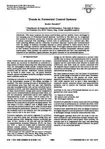
We are witnessing technological advances in VLSI, in MEMS, and in communication networks that have brought devices with sensing, processing, actuating, and communication capabilities. These devices have contributed to the formation of Networked Control Systems (NCSs) [1]. The fundamental motivation of NCSs is that they extend the distributed control of the physical world beyond distance barriers [2]; see Fig. 1. Representative applications include industrial automation, distributed instrumentation, unmanned vehicles, home robotics, distributed virtual environments, power distribution, and building structure control [3]. Successful design and implementation of NCSs necessitate the existence of simulation tools that allow verification, validation, and evaluation of different control and network algorithms. In this paper, we argue that simulation of NCSs needs to be carried out through co-simulation, which requires the joint and simultaneous simulation of both physical and communication networks dynamics. The need for co-simulation originates from the fact that the NCS field is an interdisciplinary one that combines the study of control theory and communication networks. In its simplest form, a NCS consists of a single physical system ⋆
Now at Jordan University of Science and Technology, Computer Engineering Dept., Irbid 22110 Jordan. e-mail:
[email protected]
Sensor
Controller
Actuator
Network
Controller r
Sensor+ actuator
Sensor
+ −
u Controller
Network
Actuators
Plant
y Sensors
(Controlled System)
Physical world
Fig. 1. (left) NCSs integrate sensing, processing, and actuation tasks that enable remote monitoring and control of the physical world. (right) A networked control system with one controlled system (a.k.a. plant) and one controller; both the sensor and the actuator are co-located at the plant site. Figures reproduced from [3].
and a remote controller such as the one in Fig. 1 (right). The sensor samples the values of physical quantities, writes them in a packet, and sends the packet over the network to the controller. The controller examines the received sample to generate a control signal that is then sent over the network to the actuator. Although more complex scenarios are possible, the most fundamental concern is to understand how the communication network and the NCS affect each other as a function of network traffic and topology, and in terms of NCS stability and performance. For example, NCS packets transmitted over the network will incur delays that are often time varying. A central concern is then to understand how these time-varying delays affect the performance or the stability of the NCS. On the other hand, a NCS would sample and transmit sensed data at a rate that is appropriate to achieve some performance levels. However, if this rate is higher than the network bandwidth capacity, the network becomes congested, thus leading to additional packet delays, losses, and jitter [2]. In a nutshell, the study of NCSs necessitates an integrated approach that combines the disciplines of networking and feedback control. Pursuing a pure analytical approach is likely to be intricate especially when considering multiple NCSs in a wide-area setting, e.g., the Internet. Mathematical formulation and analysis based on fixed delays and on regular sampling intervals may no longer be applicable when packets carrying sensed and control data are subject to long and time-varying delays or the possibility of being lost. Since co-simulation will at least lead to a numerically tractable analysis of the overall system, we believe that co-simulation will be critical to the study of complex systems and of scalable control algorithms in such wide-area settings. In these cases, co-simulation enables us to construct synthetic large-scale networks and workloads, to replay collected traces, and to obtain a complete snapshot of both the network behavior and the physical systems states. For these facts, co-simulation is a key step in NCS co-design, whereby network issues such as bandwidth, quantization, survivability, reliability, scalability, and message delay are considered simultaneously with controlled system issues such as stability, performance, fault tolerance, and adaptability [4]. A common feature for any co-simulation tool is that it needs to capture both the physical and the communication dynamics. For the simple example in
Fig. 1 (right), the tool simulates the physical system and derives the system output that is captured by the sensor at the sampling instances. Then, packets are simulated to traverse the network links from sensor to controller, incurring latencies and subject to the possibility of being lost. The simulated controller computes the control signal and inscribes it into a packet that is delivered over the simulated network to the actuator. Finally, the tool simulates the action taken by the actuator. The effectiveness of co-simulation relies on how well a tool describes the dynamics of both the physical systems and communication networks involved. For network dynamics, the tool needs to simulate detailed perpacket events, such as packet forwarding and transmission over communication links, as well as packet enqueueing and dequeueing at different network nodes. As for physical dynamics, the tool should allow the expression of differential algebraic equations (DAEs), be able to solve DAEs, and have the capability of catching events, e.g., zero crossing. In short, it should be capable of simulating general hybrid dynamical systems [5, 6]. In this paper, after reviewing the related work (Sect. 2), we present our approach for the NCS co-simulation in Sect. 3. Sections 4 through 6 elaborate on our approach by overviewing three tools we have developed for NCS cosimulation. For each tool, we highlight its capabilities and present demonstrative case studies. Finally, Sect. 7 concludes the paper.
2
Background and Related Work
There have been well-developed simulation tools that target the simulation of either networks or physical systems separately. For example, networks simulators include ns-2 [7] and OMNet++ [8]. On the other hand, simulations of physical and embedded systems utilize hybrid systems tools, which allow the construction and the simulation of systems involving continuous and discrete dynamics. Examples of hybrid systems simulation tools include Modelica simulation environments [6], Simulink [9], Ptolemy [10], and adevs [11]. Simulation of NCSs, which involve the interaction between communication networks and physical systems dynamics, can leverage on the previously mentioned tools. One direction is to utilize and to extend hybrid systems simulation tools to also simulate the events and dynamics of communication networks. An example of a tool that follows this approach is TrueTime [12]. However, TrueTime has support for only local-area networks simulations. Specifically, it allows the simulation of only the physical and the medium-access layers [12]. This limitation inhibits its applicability to more general networks that incorporate higher-layer network protocols, e.g., routing, transport, and application protocols, and geographically distributed networks, such as WANs. Providing support for general network settings in TrueTime can be a formidable task because such higher-protocols in general utilize complex algorithms that are distributed in nature and encompass multi-hop nodes. This same discussion applies to other tools that try to extend hybrid systems simulation tools to support network-side simulations; see for example [13], where Ptolemy was extended to simulate wire-
less sensor networks. An alternative direction is to extend a network simulator, such as ns-2, to include the capability for physical systems simulations. In Sect. 4 of this paper, we review one such tool, which is an extension of ns-2 called Agent/Plant. With Agent/Plant, physical dynamics of an environment and control algorithms can be modeled by ordinary differential equations (ODEs) and then solved within the simulation script or via a call to an outside utility, e.g., the Ode UNIX utility or Matlab. The same approach was also used in the ns-2 agents NSCSPlant and NSCSController (see Sect. 5 and [2]). A third direction is to marry a full-fledged network simulator and a full-fledged physical dynamics simulator. The integration of the two domain-specific simulators would then furnish a tool that combines the best features of the individual simulators. Such a methodology was sought in [14], where ns-2 was integrated with adevs. Although the tool was developed specifically to simulate power systems and networks, it can be applied to NCSs in general because the discrete-event simulator, adevs, can be used to simulate general hybrid systems. In Sect. 6 of this paper, we present a tool that is similar in spirit to [14], where we combine ns-2 with Modelica. However, in contrast to [14], our tool does not require deriving mathematical modeling equations for system states nor the formulation of input/output and state transition automata. Since Modelica’s simulation environments, e.g., Dymola, have the nice features of drag-and-drop and easeof-use in building physical systems models, our tool can be accessible to a wide spectrum of investigators, especially those with little background in hybrid and physical systems modeling. Independent of our research, [15] integrates ns-2 with the MoCoNet platform.
3
Our Approach
Our approach is to rely on and to combine well-established simulation tools for networks and for physical systems as much as possible. For example, for the network-side simulations, we employ ns-2 [7], which is a widespread discreteevent simulator developed to facilitate the simulation of network protocols at different layers of the Internet stack, including the MAC, network, transport, and application layers [16]. ns-2 simulates the exact dynamics and events of individual packets while traversing network elements, e.g., communication links and routers. With ns-2, different network topologies can be constructed, and several network technologies can be simulated, such as wireline, wireless, localor wide-area networks; or a hybrid of these. Although ns-2 supports some real-time applications, such as multimedia streaming protocols, it still lacks support for applications that involve real-time sensing, actuation, and control. Specifically, ns-2 lacks the ability of simulating continuous-time dynamics, supporting event-catching, and constructing models for physical systems. However, a nice feature of ns-2 is that it is evolvable in the sense that new protocols and algorithms can be added to the already existing ones. In particular, ns-2 exposes well-defined APIs that greatly facilitate developing new traffic sources, traffic destinations, and router queueing algorithms. In
Sects. 4 through 6, we discuss how to exploit this to extend ns-2 and combine it with other tools to provide the ability of simulating physical systems dynamics. For illustration, we next present a short example of setting up a network topology in ns-2. A Tcl simulation script can be written to define the network topology, to define traffic sources and destinations, and to schedule events. For example, the following Tcl snippet defines the network in Fig. 2. # Create nodes and label them set n0 [$ns node] $n0 label "Controller" set n1 [$ns node] $n1 label "Router" set n2 [$ns node] $n2 label "Plant0" # n3-nk are defined similarly here (code suppressed) # Connect the nodes with a star topology $ns duplex-link $n0 $n1 1Mb 1ms DropTail $ns duplex-link $n1 $n2 1Mb 1ms DropTail # Links connecting nodes n3-nk to n1 are # defined similarly here (code suppressed)
Plant0 2 Controller 0
Router L1 : c1 /d1
1
/d 2 : c2
L2 L3 : c3 /d3
:c k/ d k
3
.....
L n
Plant1
Plantj k
Fig. 2. A network topology consisting of several end-hosts (plants or controllers) connected via a router. Each communication link Li is characterized by the bandwidth ci and the propagation delay di . The number of plants, j, ci , and di may be varied across experiments.
To simulate network traffic, one can then attach, say, a TCP traffic source at node 0 and a TCP traffic sink at node 2, and then simulate the transfer of a virtual file from node 0 to node 1 using FTP. In the next three sections, we show how to use our contributed packages to simulate the flow of sensory and control packets to accomplish feedback control over a network simulated via ns-2.
4
The Agent/Plant Extension
To support NCS co-simulation in ns-2, we have implemented an extension of ns-2 to simulate physical dynamics and control laws, and the transmission of sensor and control packets between plants and controllers. The extension supports a new type of ns-2 agent, called Agent/Plant, that represents the interface between the physical and the network dynamics. An Agent/Plant can take the role of a sensor, a controller interface, or an actuator depending on its usage in the simulation script. Pairs of plants are connected to each other, after which they can exchange sampled data and control instructions. 4.1
Agent/Plant Usage
Agent/Plant is a generic ns-2 agent, which allows simulation of different configurations of NCSs. For example, it can be used to simulate any combination of time-driven and event-driven plants and controllers. Also, it allows simulation of various plant dynamics (e.g., continuous, discrete, linear, or nonlinear) and various corresponding controllers (e.g., P or PI). To achieve such flexibility, Agent/Plant requires two functions to be defined in the Tcl code, which are sysphy and smplschd; see [17] for fuller details. sysphy: The function sysphy is used by plants to simulate the physical dynamics of the controlled system and to apply control signals arriving from controllers (with actuators). Likewise, it is used by controllers upon receiving sensed data packets and when computing the control signals. Physical dynamics and control algorithms can be modeled by ODEs that are solved directly inside sysphy or via a call made to external utility, e.g., the Ode UNIX utility or Matlab. smplschd: The function smplschd schedules a future invocation to sample the system (sensor or controller) output. The function is especially helpful in the case of sensors to implement fixed or variable sampling-rate policies. It is also used at the controller site to trigger the transmission of control messages. 4.2
Example
A pair consisting of a plant (including a time-driven sensor and an event-driven actuator) and a corresponding event-driven controller can be instantiated and attached to nodes 2 and 0 of Fig. 2, respectively, as follows: # # # #
The two functions, sysphy and smplschd, are defined here to include dynamical equations that simulate the plant dynamics and the controller algorithm; see [17] for examples how to accomplish this.
# Create a controller agent and attach it to node n0
set c0 [new Agent/Plant] $ns attach-agent $n0 $c0 # Create a plant and attach it to node n2 set p0 [new Agent/Plant] $ns attach-agent $n2 $p0 # Connect the two agents $ns connect $c0 $p0 # Schedule events $ns at 0.1 "$p0 sample" $ns at 16.0 "finish"
4.3
Case Studies
To demonstrate the capabilities of Agent/Plant, we study the influence of the configuration and the time-dependent dynamics of a network on NCSs. Other experimental results using Agent/Plant appeared in [4, 18]. The Impact of Buffer Size. We start by considering several linear scalar plants that are connected via the network in Fig. 2 (i.e., the plants are attached to nodes 2, 3, . . ., k). Each plant is controlled by a proportional controller that is attached to node 0 (see also the sample code in Section 4.2). The plant dynamics and controller law are defined as follows: x(t) ˙ = ax(t) + u(t) ,
y(t) = x(t) ,
u = K(R(t) − y(t)) ,
(1)
where x(t) is the plant’s state; y(t) is the plant’s output; u(t) is the plant’s input that is sent by the controller; a is the plant constant; K is the controller proportional gain; R(t) is the reference trajectory the plant is required to follow. Now, we study the impact of router buffer size on the number of NCSs that can be accommodated by a given network topology. Large buffer sizes lead to long queueing delays but less packet loss; whereas small buffers sizes lead to relatively shorter queueing delays and higher packet loss rates. Because both delays and losses affect the NCSs performance and stability, buffer sizes is expected to be a critical factor on the number of NCSs that can be accommodated in particular network configurations. For the network in Fig. 2, we investigate the impact of the router’s buffer size on the number of NCSs for two cases: when the buffer size is four and when it is two. For each buffer size, we vary the number of NCSs from 1 to 39 and for each experiment, we report the packet drop rate at the router. The parameters of each NCS are as follows: a = 100; K = 101; R(t) = 1 (i.e., unit step response); the initial plant state is x(0) = 0; and the sampling interval is constant and is drawn from a uniform distribution between 5ms and 15ms. The network parameters are as follows: c1 = 1.544Mbps; d1 = 1ms. For each link Li , where i > 1, ci = 100Mbps and di = 120µs. Finally, all packet sizes are 48B. The results depicted in Figs. 3 and 4 obviously show the striking difference between the performance when using different buffer sizes.
5 Plant # 39 Output
Avg. Drop Rate (%)
16 12 8 4 0
4 3 2 1 0
0
10
20 30 # of Plants
40
0
2
4 6 8 Time (seconds)
10
0
10 20 30 # of Plants
40
1
Plant # 39 Output
30 25 20 15 10 5 0
Plant # 20 Output
Avg. Drop Rate (%)
Fig. 3. Buffer of size 4: drop rate for n = 1, . . . , 39; plant response for n = 39. Figure is reproduced from [4].
0.8 0.6 0.4 0.2 0 0
2 4 6 8 10 Time (seconds)
1.6e+33 1.2e+33 8e+32 4e+32 0 -4e+32 -8e+32 -1.2e+33 0
2 4 6 8 Time (seconds)
10
Fig. 4. Buffer of size 2: drop rate for n = 1, . . . , 39; plant response for n = 20 and for n = 39. Figure is reproduced from [4].
Experimental Sampling Period and Delay Stability Region. Agent/Plant provides the flexibility for simulating arbitrarily complicated plant dynamics and networks beyond the previous settings. In particular, Agent/Plant can be used to simulate nonlinear plant dynamics. In [19, 18], we demonstrated the strength of co-simulation by using Agent/Plant to characterize an empirical Sampling Period and Delay Stability Region (SPDSR) for a 4-dimensional pendulum-cart system. The empirical SPDSR was compared to the analytical SPDSR, which assumes fixed sampling periods, fixed delays, and no data losses.
5
The NSCSPlant and NSCSController Extensions
We developed two new ns-2 agents that are based on the Agent/Plant framework. These two agents are referred to by NSCSPlant and NSCSController, which stand for networked-sensing-and-control-systems plant and controller, respectively. NSCSPlant is an abstract agent class, which can be used to instantiate several controlled systems, each of which simulates a physical system; NSCSController can be used to instantiate controllers. NSCSPlant supports adaptive sampling policies, whereby the sampling rate is adjusted based on a utility (performance) function associated with a particular plant. The two new agents were used to study the bandwidth allocation problem in NCSs; see [2]. According to the proposed scheme in [2], routers monitor the congestion level on links and convey this information back to plants via a special header in the sensor and controller packets. NSCSPlant then regulates its
sampling rate based on the associated utility function and using the congestion information fed back from network routers. The proposed scheme of [2] achieves a fair allocation by ensuring that the aggregate utility of all NCSs is maximized. 5.1
Case Study
Consider two NCSs sharing the bottleneck link L1 of Fig. 2. The two plants and their respective controllers are governed by (1). The first NCS, ncs0 , is parameterized by a0 = 0.1, K0 = 2.0. It starts sampling (i.e., acquires the network) at time 50s, and stops at time 150s. The second NCS, nsc1 , is parameterized by a1 = 1.0, K1 = 5.0, starting time = 0s, and ending time = 100s. Each NCS transmits packets based on the following utility function Ui (ri ) =
ai − Ki ai /ri , e ai
i ∈ {0, 1} ,
where ri is the sampling (transmission) rate for ncsi (see [2] for more details). The network parameters are c1 = 1.0Mbps, d1 = 5.0ms, c2 = c3 = 10.0Mbps, d2 = d3 = 1.0ms. All packets are 100B. Both plants are required to follow R(t) shown in Fig. 5(a). Figure 5(b) shows how ncs1 adapts its transmission rate by reducing its sampling rate when ncs0 starts operating; and how ncs0 increases its sampling rate when ncs1 stops operating. The two NCSs share the bottleneck bandwidth according to their utility functions. Moreover, the allocation scheme retains 100% network utilization during all time intervals (this can be inferred by adding transmission rates of ncs0 and ncs1 during each interval). Both NCSs stay stable and track the reference signal accurately (Figs. 5(c) and 5(d)). For more experimental results utilizing the two agents NSCSPlant and NSCSController, see [20, 2, 21], where we experimented with a larger number of NCSs.
6
Modelica/ns-2 Integration
Although the Agent/Plant has much flexibility, modeling of large physical systems, especially those incorporating systems of subsystems and those including hybrid dynamics, becomes a tedious, and perhaps an error prone, task. Therefore, it would be rational to exploit any of the tools that facilitate the construction and simulation of physical systems models, and combine it with the Agent/Plant. One such tool is Modelica. Modelica is a modeling language for large-scale physical systems. It supports model construction and model reusability; supports acausal modeling; has numerous available libraries, e.g., power systems, hydraulics, pneumatics, and power train; and has available commercial and open source simulation environments [6]. Since both Modelica and ns-2 are not readily interoperable, we integrate them by creating interprocess communication interfaces in ns-2 and in Modelica. We have created a new ns-2 application that is responsible for communicating to a corresponding Modelica model. For example, the ns-2 application can receive packets in the ns-2 simulation and use their payload to set a control
2000 Tx rate (pkt/sec)
Input R(t)
0.75 0.5 0.25 0 -0.25 -0.5 -0.75
r1
1200
r0
800 400 0
0
50
100
150
0
50
100
Time (seconds)
Time (seconds)
(a)
(b)
0.75 0.5 0.25 0 -0.25 -0.5 -0.75
Plant0 state, x0(t)
Plant1 state, x1(t)
1600
0
50
100
150
0.75 0.5 0.25 0 -0.25 -0.5 -0.75 50
100
Time (seconds)
Time (seconds)
(c)
(d)
150
Fig. 5. (a) The input signal, R(t), the two plants are instructed to follow. (b) The transmission/sampling rates r0 and r1 for ncs0 and ncs1 . (c) and (d) The plants states x1 (t) and x0 (t), respectively, while tracking the input signal R(t) in (a).
signal in a corresponding Modelica actuator. On the Modelica side, we have written inter-simulator communication routines that we can link to generic sensor and actuator models. As a result, simulator communication is achieved by pairs of corresponding modules, one in each of the two simulators [22]. The Modelica/ns-2 intercommunication mechanics guarantees the synchronization between the two simulators such that events from one simulator propagate to the other at the appropriate time [22]. The intercommunication relies on UNIX named pipes and is explained in Fig. 6. In [22], this combined tool was used to simulate a NCS consisting of a power transmission system that is controlled over a wide-area network. In that scenario, the power system involved typical power grid elements, including a permanentmagnet generator, a transmission line, and time-varying loads. The scenario also included a PID controller to regulate the generator’s output voltage under varying load, using output measurements sent over the network. Our co-simulation tool enabled us to investigate the influence of network cross-traffic on the NCS’s ability to stabilize the voltage.
6.1
Case Study
In this paper, we apply our Modelica/ns-2 co-simulation tool to a NCS involving a drive train that is controlled by a PI controller (see Fig. 7). The model is constructed using blocks from the Modelica standard library plus our new Network block that communicates with ns-2.
ns−2
Modelica
Start at simulation time t 0
Start at simulation time t 0
Run until application needs to communicate (at simulation time t)
Instructed by ns−2 to progress?
No Instruct Modelica to run until simulation time t
Read from or Write to pipe
Yes Run until simulation time t
Write to or Read from pipe
Fig. 6. The Modelica/ns-2 intercommunication mechanics. ns-2 runs first and Modelica is paused. When the ns-2 application is slated by ns-2’s event scheduler to receive (deliver) data from (to) a Modelica model at time t, it instructs Modelica to run until time t, and to exchange data at that point. After the data exchange, Modelica simulation time is suspended until the ns-2 application is scheduled again. Dashed lines represents communication via UNIX named pipes.
For the scenario in Fig. 7, the objective is to control the motor inertia (Inertia1) to follow the reference speed signal shown in Fig. 8. The reference speed is generated by the two blocks KinematicPTP and Integrator. The output of the controller is a torque that drives Inertia1. The load inertia, Inertia2, is attached to Inertia1 via a compliant spring-damper component. Also, there is a constant external torque of 10Nm acting on the load inertia. The speed measurements from Inertia1 are transported to the PI controller over a communication link that is shared with other traffic flows. Finally, Network is our newly developed Modelica block that contains the inter-simulator routines to allow Modelica models to communicate with ns-2. Now, assume that the packets carrying the speed measurements flow from node 2 to node 0 of the network in Fig. 2. In this example, the network exists only in the feedback path that connects the plant to the controller but not in the forward path that connects the controller to the plant. Furthermore, we assume that the link L1 is also traversed by cross-traffic corresponding to a multimedia application whose source and destination are attached to nodes 3 and 0, respectively. The network parameters are the same as those in Sect. 5. The speed is sampled at constant intervals of 2ms, and the samples are inscribed into packets of size 100B. The multimedia source starts injecting packets in the network at time 2sec and lasts for only 1sec. The multimedia packets are 1000B. We consider the effect of cross-traffic on the drive train NCS for two cases: when the multimedia source transmits at a constant rates of 625Kbps and 715Kbps.
Fig. 7. A drive train NCS created by inserting our Network block into an example system that is part of the Modelica standard library [6]. The plant is a cascade of five mechanical elements: Torque, Inertia1, Spring, Inertia2, and LoadTorque. The Plant is controlled by a PI controller, PI, to follow the reference speed generated by the two blocks KinematicPTP and Integrator. The SpeedSensor measures the speed of Inertia1 at fixed sampling intervals. Network is responsible for communicating back and forth with ns-2 to relay and receive packets.
Figure 9 shows the speed of Inertia1, i.e., ω in Fig. 7, for these two cases. Obviously, the multimedia rate of 715Kbps leads to more contention between multimedia and NCS packets than that of 625Kbps. When the aggregate rate of both the NCS and of the multimedia traffic exceeds c1 , packets are enqueued in the router buffer (see Fig. 10). As a result, queueing delays deteriorate the control performance and jeopardize the NCS’s stability.
1.25 1 0.75 0.5 0.25 0 -0.25 0
1
2 Time (seconds)
3
4
Fig. 8. The reference speed that Inertia1 is required to follow.
1.2
1
625Kbps ω (rad/sec)
0.9
0
0.6 -1 0.3 -2 715Kbps
0 0
1
2
3
4
0
1
2
3
4
Time (seconds)
Queue Size (packets)
Fig. 9. The speed of Inertia1, i.e., ω in Fig. 7, when the multimedia application sends packets at a constant rate of 625Kbps and 715Kbps. 18 15 12 9 6 3 0
72 60 48 36 24 12 0
625Kbps
0
1
2
3
4
715Kbps
0
1
2
3
4
Time (seconds)
Fig. 10. The queue length at the router of Fig. 2 for the two cases when the multimedia application sends packets at a constant rate of 625Kbps and 715Kbps.
7
Conclusions
We overviewed three tools that we have developed for the co-simulation of Networked Control Systems (NCSs). All of our tools use ns-2 to simulate the communication networks side. The first two tools require modeling of and deriving equations for physical dynamics. Our newly developed tool integrates Modelica with ns-2 so it reduces physics modeling time, effort, and errors. We argued that co-simulation is indispensable to the study and further progress of NCSs because NCSs, in general, involve hybrid and time-varying dynamics, thus making pure analytical approaches intractable in large scale configurations. That said, we have not examined the scalability or optimality of our proposed co-simulation paradigm. Specifically, one should examine how the computation time and memory usage of co-simulation scale as the number of plant models and their complexity increase. These matters are the subject of future research.
Acknowledgments Research supported in part by NSF CCR-0329910, Department of Commerce TOP 39-60-04003, and Department of Energy DE-FC26-06NT42853.
References 1. Zhang, W., Branicky, M., Phillips, S.: Stability of networked control systems. IEEE Control Systems Magazine 21(1) (2001) 84–99 2. Al-Hammouri, A.T., Branicky, M.S., Liberatore, V., Phillips, S.M.: Decentralized and dynamic bandwidth allocation in networked control systems. In: Proc. Intl. Workshop Parallel and Distributed Real-Time Systems, Rhodes, Greece (2006) 3. Liberatore, V.: Integrated play-back, sensing, and networked control. In: Proc. of IEEE INFOCOM. (2006) 4. Branicky, M.S., Liberatore, V., Phillips, S.M.: Networked control system cosimulation for co-design. In: Proc. American Control Conf., Denver (2003) 5. Branicky, M., Mattsson, S.: Simulation of hybrid systems. In Antsaklis, P., et al., eds.: Hybrid Systems IV, Lecture Notes in Computer Science. Volume 1273., Berlin (1997) 31–56 6. Modelica and Modelica Association. ([Online]. Available: http://www.modelica.org) 7. Network Simulator—ns-2. ([Online]. Available: http://www.isi.edu/nsnam/ns) 8. OMNeT++: Discrete Event Simulation System. ([Online]. Available: http://www.omnetpp.org) R version 6.1. The MathWorks Inc.: (2004) 9. Simulink 10. The Ptolemy Project. ([Online]. Available: http://ptolemy.eecs.berkeley.edu) 11. ADEVS: A Discrete EVent System simulator. ([Online]. Available: http://www.ornl.gov/∼1qn/adevs/index.html) 12. Cervin, A., Ohlin, M., Henriksson, D.: Simulation of networked control systems using TrueTime. In: Proc. International Workshop on Networked Control Systems: Tolerant to Faults, Nancy, France (2007) 13. Baldwin, P., Kohli, S., Lee, E.A., Liu, X., Zhao, Y.: Modeling of sensor nets in Ptolemy II. In: Proc. Info. Processing in Sensor Networks, Berkeley, CA (2004) 14. Nutaro, J., Kuruganti, P.T., Miller, L., Mullen, S., Shankar, M.: Integrated hybridsimulation of electric power and communications systems. IEEE Power Engineering Society General Meeting (2007) 1–8 15. Nethi, S., Pohjola, M., Eriksson, L., Jantti, R.: Platform for emulating networked control systems in laboratory environments. In: IEEE Intl. Symp. World of Wireless, Mobile and Multimedia Networks, Espoo, Finland (2007) 16. Kurose, J.F., Ross, K.W.: Computer Networking: A Top-Down Approach Featuring the Internet. Addison Wesley Longman, Inc. (2001) 17. Liberatore, V.: Agent/Plant extension. ([Online]. Available: http://vorlon.case.edu/∼vxl11/NetBots) 18. Hartman, J.R., Branicky, M.S., Liberatore, V.: Time-dependent dynamics in networked sensing and control. In: Proc. American Control Conf., Portland (2005) 19. Hartman, J.: Networked control system co-simulation for co-design: Theory and experiments. Master’s thesis, Case Western Reserve Univ., Cleveland, Ohio (2004) 20. Al-Hammouri, A.T., Liberatore, V.: Optimization congestion control for Networked Control Systems. In: Proc. of IEEE INFOCOM Student Workshop, Miami, FL (2005) Abstract. 21. Al-Hammouri, A.T.: Internet Congestion Control: Complete Stability Region for PI AQM and Bandwidth Allocation in Networked Control. PhD thesis, Case Western Reserve Univ., Cleveland, Ohio (2008) 22. Al-Hammouri, A.T., Liberatore, V., Al-Omari, H., Al-Qudah, Z., Branicky, M.S., Agrawal, D.: A co-simulation platform for actuator networks. In: Proc. ACM Conference on Embedded Networked Sensor Systems, Sydney (2007) Demonstration.