Sep 29, 2008 - to classify and track the vehicles. Our goal in this paper is to segment a multi-vehicle blob (a binary mask) into some single-vehicle blobs. Fig.
Author manuscript, published in "The Eighth International Workshop on Visual Surveillance - VS2008, Marseille : France (2008)"
Co-Training Based Segmentation of Merged Moving Objects Tianzhu Zhang, Stan Z.Li, Shiming Xiang, Lun Zhang, Si Liu Center for Biometrics and Security Research & National Laboratory of Pattern Recognition Institute of Automation,Chinese Academy of Science 100190,Beijing,P.R.China {tzzhang,szli,smxiang,lzhang,sliu}@cbsr.ia.ac.cn
inria-00325626, version 1 - 29 Sep 2008
Abstract Object detection and tracking are basic tasks in video surveillance and have been an active research area. Using a standard Gaussian Mixture Model (GMM) based method, nearby objects could be merged into a single foreground object. This causes difficulties in foreground segmentation, especially when objects in the foreground have similar in color, texture and shape. This paper proposes a novel method for segmenting merged objects into individual ones. First, an unsupervised co-training framework is proposed for the detection of foreground containing multiple vehicles. The co-training based approach is to simultaneously train two disparate classifiers based on independent features. One is a naive Bayes classifier based on scene context features, such as direction of motion and width of vehicles; the other is an appearance classifier based on Multi-block Local Binary Pattern (MB-LBP) features. Unlabeled examples which are confidently labeled by one classifier are added, with labels, to the training set of the other classifiers. The trained classifiers are then used to classify detected foregrounds into containing either a single vehicle or multiple vehicles. As the second step, foreground containing multiple vehicles is further segmented into individual vehicles by means of projection histogram analysis. Experimental results show the effectiveness and efficiency of the proposed framework.
1. Introduction Object detection and tracking are basic tasks for intelligent video surveillance. When using stationary cameras, background subtraction is a widely used technique for extracting moving pixels (foreground). If there are several objects in the scene, each connected component of the foreground (blob) usually corresponds to an object, such a blob is denoted as single-vehicle blob. However, it can happen that several objects form one enlarged blob, which we call
Figure 1. Some examples of single-vehicle blobs and multi-vehicle blobs. The red boxes are the results of GMM detector. The blue boxes segment the multi-vehicle blobs into single-vehicle blobs using our algorithm.
a multi-vehicle blob, caused by view at an angle, shadow and nearby moving vehicles. Since a multi-vehicle blob is detected as one foreground, it is difficult to obtain the appearance feature of each single vehicle. Thus it is difficult to classify and track the vehicles. Our goal in this paper is to segment a multi-vehicle blob (a binary mask) into some single-vehicle blobs. Fig. 1 illustrates an example. To solve this problem we take two steps. First, a classifier is used to classify the foreground into either a singlevehicle blob or a multi-vehicle blob. The second step is to segment the multi-vehicle blob into single-vehicle blobs. Currently the popular method for training the image classifier is to adopt a semi-supervised learning algorithm from a combination of both labeled and unlabeled data. Semisupervised learning provides a general framework to learn a classifier for different types of objects which may not have enough labeled data. Some examples of semi-supervised learning algorithms include: the Expectation-Maximization (EM) algorithm [2], co-training [1], tri-training [22], and transductive support vector machine [8]. One typical algorithm is the co-training approach pro-
inria-00325626, version 1 - 29 Sep 2008
posed by Blum and Mitchell [1]. The basic idea is to train two classifiers on two independent “views ”(features) of the same data, using a relatively small number of examples. Unlabeled examples are then fed to these classifiers and labeled (classified). The most confidently labeled examples from one classifier are then added to the labeled set of the other classifier. In other words, the classifiers train each other using the unlabeled data. Blum and Mitchell prove that co-training can find a very accurate classification rule, starting from a few labeled examples if the two feature sets are statistically independent. However, the assumption therein is found unlikely to hold in most real world cases [13]. On the other hand, Levin et al. [9] build boosting classifiers for gray-image and background difference features which co-train each other to improve the overall detection performance. Note that the features used by Levin et al. [9] are closely related. Nonetheless, their approach empirically proves that co-training is still possible even in the case the independence assumption does not hold. Other work on learning using co-training framework follow subsequently. Nair et al. [11] proposed an unsupervised learning approach for human detection which uses motion information as an “automatic labeler” to supply labeled training examples. Such an algorithm only works under restricted conditions. Javed et al. [7] proposed to improve an off-line learned object detector using co-training based on Principal Component Analysis (PCA) features. A constraint is that it needs a pre-trained classifier which limits its capability to be generalized to arbitrary object types. On the other hand, this work also deal with segmenting a multi-vehicle blob into individual ones. Some works have been proposed to solve the crowd segmentation problem, which emphasize on locating individual humans in a crowd. In [6, 20], head detection is used to help locate the position of humans. Rittscher et al. [14] have developed a method based on partitioning a given set of image features using a likelihood function that is parameterized on the shape and location of potential individuals in the scene. They use a variant of the Expectation Maximization (EM) algorithm [2] to perform global annealing based optimization and find maximum likelihood estimates of the model parameters and the grouping. Dong et al. [3] propose a novel example-based algorithm which maps a global shape feature by Fourier descriptors to various configurations of humans directly and use locally weighted average to interpolate for the best possible candidate configuration. In addition, they use dynamic programming to mitigate the inherent ambiguity. Zhao and Nevatia [20] use human shape to interpret foreground in a Bayesian framework. However, these mentioned methods are not appropriate for segmenting a group of vehicles into individual. Because directions of motion of vehicles are different, their postures will change, which cause these features are not feasible. In ad-
Figure 2. The proposed framework for multivehicle blob segmentation.
dition, vehicles in a group may have similar color, texture and shape features. This paper proposes a novel method for segmenting merged objects into individual ones. This is accomplished in two steps: (1) classifying each foreground blob into either multi-vehicle blob or single-vehicle blob, and (2) segmenting a multi-vehicle blob into individual ones. Figure 2 illustrates the framework. A simple background subtraction based on on-line Gaussian Mixture Model (GMM) [15] is used to detect the moving objects. Then the moving pixels are connected to obtain blobs. For each blob, a classifier is adopted to classify it into single-vehicle blob or multivehicle blob. If the blob is multi-vehicle blob, it will be segmented into some single-vehicle blobs based on scene context features. Then the single-vehicle blob is tracked and classified at the next step. For the first step, we propose an unsupervised method for learning two classifiers for the classification of a foreground into a single-vehicle blob or a multi-vehicle blob, inspired by the idea of co-training learning. Two sets of features are predefined and they are relatively independent of each other: (1) scene context features, such as direction of motion and width of vehicles; and (2) appearance features based on Multi-block Local Binary Pattern (MB-LBP) [10, 19]. Two labeled sets are then prepared based on them, each for training one of the classifiers. A currently trained classifier classifies unlabeled examples to obtain their labels and add those newly labeled examples which are confident enough to update the other training set for a new classifier training. In applications, the outputs of the two classifiers are combined to give the final classification decision. Experiments demonstrate that co-training can generate an accurate classifier conveniently and effectively. For the second step, we propose a method based on scene
context features to solve this problem. These features reflect motion rules of vehicle. Once these features are obtained, direction of motion and size of vehicle at a certain location can be estimated. Experiments demonstrate efficiency of our method. The rest of the paper is organized as follows: Section 2 introduces the method to learn the scene context features. The proposed unsupervised learning framework based on co-training is presented in section 3. A simple method to segment multi-vehicle blob into single-vehicle blobs is introduced in section 4. Section 5 shows some results. Finally, we conclude the paper in section 6.
inria-00325626, version 1 - 29 Sep 2008
2. Learning Scene Context Features Scene context features reflect the properties of objects in the scene image, they can be used to distinguish objects. it is time-consuming and needs a lot of storage space to obtain these features for each pixel in the scene image. Adjacent pixels in scene image have similar scene context features, therefore, it is viable to cut the scene image into R × C fixed blocks, R is the number of row and C is the number of column. The size of each block is relatively small, hence the direction of motion and size of a moving object in a certain block is viewed to be constant. Therefore, the method to learn scene context features based on each block is feasible. Direction of motion of vehicles can be obtained by analyzing their trajectories, then the direction of motion in each block can be learnt by using direction of vehicles. After obtaining the direction in each block, width distribution in each block can be learnt by using width of vehicle which is extracted by projecting its binary mask onto the direction that is perpendicular to the direction of motion in each block.
2.1. Learning Direction of Motion A trajectory can be obtained by tracking the centroid of an object, in the 2-D image coordinates, whose origin is on the bottom left corner, it can be described as T = {(x1 , y1 ), (x2 , y2 ), · · · , (xn , yn )}. In general traffic scenes, trajectory of a vehicle is not complicated, thus it is reasonable to use quadratic curve (y = a×x2 +b×x+c) to describe the trajectory. The parameters (a, b, c) are its features. For a tracked object, all points from start point to end point are collected to calculate the parameters (a, b, c) by least squares fit to the y values. Therefore, the parameters (a, b) which express the motion direction of the vehicle are obtained. Fig. 5(b) shows the parameters in each block. Because there are many clutter trajectories, the distribution of parameters (a, b, c) in each block are represented by multiple Gaussian models, which can be described as follows:
Each block in the scene is modeled by a mixture of K Gaussian distributions for trajectory parameters. For a certain block at position (x0 , y0 ) of the scene image, the series of trajectories {Tt = (at , bt , ct )}N t=1 are obtained. Here (at , bt , ct ) are parameters of a trajectory Tt . They are used to learn the parameters distribution of blocks which the object has passed. The probability that a certain block has a value of Tt at time t can be written as P (Tt ) =
K X
wi,t × η(Tt , ui,t , Σi,t )
(1)
i=1
where wi,t is the weight parameter of the ith Gaussian component at time t, η(Tt , ui,t , Σi,t ) is the ith Normal distribution of component with mean ui,t and covariance Σi,t . Here Σi,t is assumed to be diagonal matrix. While this is certainly not the case, the assumption allows us to avoid a costly matrix inversion at the expense of some accuracy. ui,t = (uai,t , ubi,t , uci,t )T
(2)
a b c T σi,t = (σi,t , σi,t , σi,t ) a σi,t 0 0 1 b 2 0 Σi,t = 0 σi,t c 0 0 σi,t
(3) (4)
The K distributions are ordered based on the fitness value wi,t . Parameters u and σ for unmatched distributions remain the same. The first Gaussian component that matches the test trajectory will be updated by the following update equations, wi,t = (1 − α)wi,t−1 + α(Mi,t )
(5)
where Mi,t is 1 for the model which matched and 0 for the remaining models. ui,t = (1 − ρ)ui,t−1 + ρTt
2 2 σi,t = (1 − ρ)σi,(t−1) + ρ(Tt − ui,t )T (Tt − ui,t )
ρ = αη(Tt |ui,t , σi,t ) th
(6)
(7)
(8)
where wi,t is the i Gaussian component, 1/α defines the time constant which determines change. If none of the K distributions match that trajectory value, the least probable component is replaced by a distribution with the current value as its mean, an initially high variance, and a low weight parameter. In our experiments, K is 3, α is 0.1, the initial high variance of (a, b, c) are (0.05, 0.2, 20), the low weight is 0.05.
2.2. Learning Width Distribution After obtaining motion direction for each block, width distribution for each block can be learnt. For a foreground with width wt in block (x0 , y0 ) at time t, the width of the foreground is used to learn the width distribution for the block. In practice, a foreground may be a single-vehicle blob or a multi-vehicle blob, their width may have significant difference. Therefore, in each block, the probabilistic distribution of the width is modeled as a Gaussian Mixture Model (GMM). We take each of the Gaussian components as one of the underlying width distribution and update the GMM parameters with adaptive weights in an online way just as the process of learning motion direction for each block. The parameters (mean wu and variance wσ ) of Gaussian component with the maximum weight are considered as the features of each block.
inria-00325626, version 1 - 29 Sep 2008
3. Moving Vehicle Classification 3.1. Naive Bayes Classifier The width of a foreground at time t is denoted by xt . The naive bayes Classifier is to decide if the foreground belongs to multi-vehicle (MV) blob or single-vehicle (SV) blob. Bayesian decision L is made by: P (M V |xt ) p(xt |M V )P (M V ) = (9) P (SV |xt ) p(xt |SV )P (SV ) In a general case we do not know anything about the foreground objects that can be seen nor when and how often they will be present. Therefore we set P (M V ) = P (SV ). We decide then that the foreground belongs to a multivehicle blob if: L=
p(xt |M V ) > L × p(xt |SV )
(10)
We will refer to p(x|M V ) and p(x|SV ) as the models. The models are estimated from a training set denoted as X and Y respectively. The estimated models are denoted by pˆ(x|X , M V ) and pˆ(x|Y, SV ) which depend on the training set as denoted explicitly. We assume that the samples are independent and the main problem is how to efficiently estimate the density function and to adapt it to possible changes. In order to guarantee the performance of Bayes classifier, We use GMM with M components: pˆ(x|X , M V ) =
M X
2 w ˆm ηˆ(x; u ˆm , δˆm I)
(11)
w ˆn ηˆ(x; u ˆn , δˆn2 I)
(12)
m=1
pˆ(x|Y, SV ) =
M X n=1
where u ˆ1 , · · · , u ˆM are the estimates of the means and δˆ1 , · · · , δˆM are the estimates of the variances that describe the Gaussian components. In our experiment, M is 2. The covariance matrices are assumed to be diagonal and the identity matrix I has proper dimensions. The parameters are updated as the same as the Equ.( 5), ( 6) and ( 7).
3.2. Appearance Based Classifier The Bayes classifier is constructed by using scene context features, however, a single-vehicle blob with large width may be misclassified into a multi-vehicle blob. Therefore, An appearance classifier based on Multi-block Local Binary Pattern (MB-LBP) [10, 19] features is adopted to improve the performance of classification. MB-LBP is extended from the original LBP feature [12], which has been proven to be a powerful appearance descriptor with computational simplicity. Besides, this feature is also successfully applied in many low resolution image analysis tasks [5]. However, it is limited to calculate the information in a small region and has no ability to capture large-scale structures of objects. MB-LBP is developed on image patches divided into sub-blocks (rectangles) with different sizes. This treatment provides a mechanism for us to capture appearance structures with various scales and aspect ratios. Intrinsically, MB-LBP is to measure the intensity differences between sub-blocks in image patches. Calculation on blocks is robust to noises, lighting changing. At the same time, MB-LBP can be computed very efficiently by using integral images [17]. The feature set of MB-LBP feature is large and contains much redundant information. AdaBoost algorithm is used to select significant features and construct a binary classifier. The gentle adaboost [4, 16] is adopted for the reason that it is simple to be implemented and numerically robust. Given a set of training examples as {(x1 , y1 ), ..., (xN , yN )}, where yi ∈ {+1, −1} is the class label of the example xi ∈ Rn . Boosting learning provides a sequential PMprocedure to fit additive models of the form F (x) = m=1 fm (x). Here fm (x) are often called weak learners, and F (x) is called a strong learner. Gentle adaboost uses adaptive Newton steps for minimizing the cost function: J = E[e−yF (x) ], which corresponds to minimizing a weighted squared error at each step.
3.3. Classifier Co-Training To train the classifiers, labeling a large training set by hand can be time-consuming and tedious. The difficulty is the high cost of acquiring a large set of labeled examples to train the two classifiers. Of course, gathering a large number of unlabeled examples in most applications has much lower cost, as it requires no human intervention. One typi-
inria-00325626, version 1 - 29 Sep 2008
cal algorithm is the co-training method which has two classifiers that train each other using unlabeled data. In our algorithm two relatively independent features are used: scene context features and MB-LBP features as the object representation. Each feature is used to train an classifier, and their outputs are combined to give the final classification results. For a data set, the Bayes classifier is initialized on-line using scene context features. For a foreground with width xt at block (x0 , y0 ) in scene image, scene context features (the mean wu and variance wσ of width) of this block can be used to classify the foreground into multi-vehicle blob or single-vehicle blob. In practice, a foreground is usually a single-vehicle blob. Therefore, the primary distribution of width in each block reflects width distribution of singleu > T h is right, the foreground is a vehicle blob. if xtw−w σ multi-vehicle blob, then update the parameters of the model pˆ(x|X , M V ), otherwise update the model pˆ(x|Y, SV ). T h is a given threshold. Once these models are learned, they can be used to label samples to train the appearance-based classifier, then add these examples to the training set and retrain the Bayes classifier. New models are then estimated. This process can be repeated many times. The main advantages of this scheme are: (1) It is a collaborative approach that uses the strength of different views of the object to help improve each other, hence a more robust classification. (2) Manual labeling is not necessary. Experiments demonstrate that co-training can generate accurate classifiers. After training the two classifiers, the final classification results of their outputs follow the rules in Table 1. Bayes Classifier SV SV MV MV
Appearance Classifier SV MV SV MV
final result SV SV SV MV
Table 1. Decision rules of the two classifiers.
4. Multi-Vehicle Segmentation Shape feature has been used to segment and localize individual humans in a crowd [3, 6, 14, 20]. However, it is difficult to simply use shape feature to segment vehicles in video surveillance. For example, Fig. 3(b) explains the reason. If we do not know the motion direction of vehicle, we are not sure whether a square shaped blob contains multiple vehicles or not. as for a vehicle, its length is longer than its width. If the direction of motion is the direction of the green line, the foreground like a single-vehicle blob. If the direction of motion is the direction of the red line, the foreground likes a multi-vehicle blob. In addition, vehicles in
a blob may have similar color, texture and shape features, therefore, it is difficult to segment a blob into individual vehicles using these features. In a fixed scene, scene context features (such as direction of motion and width distribution of vehicles)are stable. These features are helpful to segment multi-vehicle blob. Therefore, this paper proposes a novel method based on scene context features to improve vehicle detection accuracy.
(a)
(b)
(c)
(d)
Figure 3. (a) The results of GMM detector. (b) The binary mask of the blob. The red and green line indicate two different directions of motion separately. (c) Vertical projection histogram of the blob. (d) The multi-vehicle blob is segmented by blue boxes using our algorithm. For a multi-vehicle blob, its vertical projection histogram [6, 21] h(x) can be obtained by projecting its binary mask onto the direction that is perpendicular to the direction of motion. To obtain the junctions of vehicles conveniently, the vertical projection histogram is smoothed to construct f (x).
f (x) =
N x − xi 2 1 X (h(xi ) × exp(−( ) )) N i=1 wu
(13)
where wu is the mean width of vehicle in the block which the foreground is inside. Table 2 is our algorithm framework. For each scene, scene context features are learnt in each block by the GMM algorithm. the learnt context features are used to initialize the Bayes classifier. Then two classifiers based on independent features are trained using co-training framework. For a foreground, if it is classified as a multi-vehicle blob, the segmentation module will run. Finally, each of single-vehicle objects is segmented from the foreground blob.
5. Experimental Results 5.1. Learning Scene Context Features Direction of motion and width of vehicle are adopted to learn scene context features for each block. As showed in figure 4, tracking a vehicle from the entry point to exit point,
For each scene 1. Learn scene context features for each block (Section 2) (a) Use vehicle’s trajectory learning direction of motion of vehicle for each block. (b) Use vehicle’s width learning width distribution of vehicle for each block. 2. Classify moving vehicle (Section 3) (a) Initialize the Bayes classifier using scene context features. (b) Train the Bayes classifier and the appearance classifier using co-training. (c) Classify each blob using the two classifiers.
Figure 6. Some examples of training samples. The training set contains single-vehicle blobs and multi-vehicle blobs, which are collected in diverse camera viewing angles.
3. If the blob is a multi-vehicle blob: Run the segmentation module (Section 4).
5.2. Object Classification
inria-00325626, version 1 - 29 Sep 2008
Table 2. Algorithm Framework
then fit the trajectory to get direction of motion for each block which the vehicle has passed. As for the blocks the vehicle has passed, the direction of motion in the each block is used to get width of the vehicle, then the width is used to learn the width distribution for the block. These context features for each block are learnt by the GMM algorithm. Some results are illustrated in Fig. 5. The scene image is cut into multiple blocks in Fig. 5(a) to learn those context features. In our experiments, R and C are both set 8 for a 320 × 240 image resolution. The direction of motion and mean width of vehicle in each block is displayed in Fig. 5(b) and 5(c) respectively. For blocks which vehicle has not passed, their features are 0. The GMM algorithm updates weight in an online way, which guarantees the primary distribution for each block can be learnt. This results suggest that our approach is effective. 14 12 10 8 6 4 2 0 0
(a)
(b)
(c)
5
10
15
20
25
(d)
Figure 4. Motion features of a vehicle. (a) A vehicle is detected. (b) The direction of motion of the vehicle. (c) The binary mask of the vehicle. (d) Vertical projection histogram of the vehicle, the number of bins is the width of the vehicle.
30
We implemented real-time background subtraction and tracking as [15, 18], so that moving objects can be reasonably separated from background and blobs can be obtained. For each scene, scene context features are learnt and the Bayes classifier is initialized on-line, then we use the classifier labeling the unlabeled samples to enlarge the training set of the appearance classifier. These samples are obtained by normalizing blobs to 20 × 20. We collected samples per 10 frames in order to reduce the correlation between vehicles. Then these samples are adopted to train the appearance classifier. Once the appearance classifier is trained, we use each classifier’s prediction on the unlabeled samples to enlarge the training set of the other. The learning process is applied to different scenes and a great number of samples are collected. The sample set consists of 79, 175 single-vehicle blobs and 12, 808 multi-vehicle blobs. Some samples are showed in Fig. 6, which represent multi-view vehicles. To test the performance of the classifiers, we collect 988 vehicle tracked sequences from 8 different scenes shown in Fig. 8. The vehicles in these test sequences are all not included in the training set. A simple voting method to the tracked sequence is used to get a final class label. Table 3 shows the classification results. This results suggest that our approach achieves considerable performance in diverse scenes.
M-Vehicle S-Vehicle
Tracks 785 203
Correct Classification 719 191
Correct Rate 91.59% 94.09%
Table 3. The classification results on test.
(a)
(b)
(c)
inria-00325626, version 1 - 29 Sep 2008
Figure 5. (a) The scene is cut into 8 × 8 blocks. (b) The value of direction of motion b in each block. Because the road is straight line, the parameter a is 0. (c) The mean of width in each block.
5.3. Object Segmentation
7. Acknowledgements
For a foreground, once it is classified as a multi-vehicle blob, the segmentation module will be started up. Supposing the foreground is inside a certain block, and the direction of motion and width distribution of vehicles in the block are used to obtain the vertical projection histogram of the foreground. Segmented boxes (blue boxes) could be obtained by finding troughs of the vertical projection histogram together with making use of the direction of motion in corresponding block. Some results about vertical projection histogram h(x) and f (x) are given in Fig. 3(c), 7(c) and 7(f). We test our algorithm in eight scenes, and collect video images randomly. There are 11365 multi-vehicle blobs in these images, and 10797 of them have been segmented into singlevehicle blobs correctly. The segmentation correct rate is about 95.0%. Some results of segmentation are showed in Fig.8. In these figures, red boxes are detected by the GMM algorithm, and blue boxes are the results of our segmentation. they validate the performance of segmentation.
This work was supported by the following funds: Chinese National Natural Science Foundation Project #60518002, Chinese National 863 Program Projects #2006AA01Z192, #2006AA01Z193, and #2006AA780201-4, Chinese National Science and Technology Support Platform Project #2006BAK08B06, and Chinese Academy of Sciences 100 people project, and AuthenMetric R&D Funds. The author would like to thank Xiaotong Yuan, and Ran He for their comments on the paper.
6. Conclusions In video surveillance, it is desirable to segment each multi-vehicle blob into single-vehicle blobs. We have proposed an effective unsupervised learning framework for solving this problem. First, classifier is adopted to classify the foreground into multi-vehicle blob or not. Then scene context features are used to segment multi-vehicle blob into individual vehicles. To train classifiers, a co-training based framework is proposed, different features of vehicle have been adopted. The segmentation framework is real-time for a 320 × 240 image resolution on a P4 3.2GHz PC, and the processing time is less than 0.1s/frame. Experimental results validate the effectiveness and efficiency of our framework. Currently, some disturbances (such as shadows) affect the performance of the segmentation. This will be improved through object detection in the future work.
References [1] A. Blum and T. Mitchell. Combining labeled and unlabeled data with co-training. In COLT: Proceedings of the Workshop on Computational Learning Theory, Morgan Kaufmann Publishers, pages 92–100, 1998. [2] A. P. Dempster, N. M. Laird, and D. B. Rubin. Maximum likelihood from incomplete data via the em algorithm. Journal of the Royal Statistical Society. Series B (Methodological), 39:1–38, 1977. [3] L. Dong, V. Parameswaran, V. Ramesh, and I. Zoghlami. Fast crowd segmentation using shape indexing. IEEE Conference on ICCV, pages 1–8, Oct. 2007. [4] J. Friedman, T. Hastie, and R. Tibshirani. Additive logistic regression: A statistical view of boosting. In Annals of Statistics, 2000. [5] A. Hadid, M. Pietikainen, and T. Ahonen. A discriminative feature space for detecting and recognizing faces. IEEE Conference on CVPR, 2:II–797–II–804 Vol.2, 2004. [6] I. Haritaoglu, D. Harwood, and L. S. Davis. W4: Real-time surveillance of people and their activities. IEEE Trans. on PAMI, 22:809–830, Aug 2000. [7] O. Javed, S. Ali, and M. Shah. Online detection and classification of moving objects using progressively improving detectors. In CVPR, pages 696–701,, 2005. [8] T. Joachims. Transductive inference for text classification using support vector machines. In Proceedings of ICML-99, pages 200–209, 1999.
(a)
(b)
(c) h(x)
f(x)
10 1.5
8 6
1
4 0.5 2 0 0
(d)
(e)
20
40
0 0
20
40
(f)
inria-00325626, version 1 - 29 Sep 2008
Figure 7. The result of GMM detector is masked by red boxes, The result of segmentation is masked by blue boxes. (b) and (e) The binary mask. (c) and (f) vertical projection histogram.
Figure 8. Some results of segmentation in the eight scenes. [9] A. Levin, P. Viola, and Y. Freund. Unsupervised improvement of visual detectors using co-training. IEEE Conference on ICCV, pages 626–633 vol.1, Oct. 2003. [10] S. Liao, X. Zhu, Z. Lei, L. Zhang, and S. Z. Li. Learning multi-scale block local binary patterns for face recognition. In ICB, pages 828–837, Seoul, Korea, 2007. [11] V. Nair and J. J. Clark. An unsupervised, online learning framework for moving object detection. IEEE Conference on CVPR, 02:317–324, 2004. [12] T. Ojala, M. Pietikainen, and D. Harwood. A comparative study of texture measures with classification based on feature distributions. Pattern Recognition, pages 51–59, 1996. [13] D. Pierce and C. Cardie. Limitations of co-training for natural language learning from large datasets. In Proceedings of the 2001 Conference on Empirical Methods in Natural Language Processing, pages 1–9, 2001. [14] J. Rittscher, P. Tu, and N. Krahnstoever. Simultaneous estimation of segmentation and shape. IEEE Conference on CVPR, 2:486–493 vol. 2, June 2005. [15] C. Stauffer and W. E. L. Grimson. Learning patterns of activity using real-time tracking. IEEE Trans. on PAMI, 22(8):747–757, August 2000.
[16] A. Torralba, K. Murphy, and W. Freeman. Sharing features: efficient boosting procedures for multiclass object detection. IEEE Conference on CVPR, 2:II–762–II–769 Vol.2, 2004. [17] P. Viola and M. Jones. Rapid object detection using a boosted cascade of simple features. IEEE Conference on CVPR, 1:I–511–I–518 vol.1, 2001. [18] T. Yang, Q. Pan, J. Li, and S. Li. Real-time multiple objects tracking with occlusion handling in dynamic scenes. IEEE Conference on CVPR, 1:970–975 vol.1, June 2005. [19] L. Zhang, S. Li, X. Yuan, and S. Xiang. Real-time object classification in video surveillance based on appearance learning. IEEE International Workshop on Visual Surveillance, in conjunction with CVPR, pages 1–8, June 2007. [20] T. Zhao and R. Nevatia. Bayesian human segmentation in crowded situations. IEEE Conference on CVPR, 02:459, 2003. [21] T. Zhao, R. Nevatia, and F. Lv. Segmentation and tracking of multiple humans in complex situations. IEEE Conference on CVPR, 2:194, 2001. [22] Z. Zhou and M. Li. Tri-training: exploiting unlabeled data using three classifiers. Knowledge and Data Engineering, IEEE Transactions on, 17:1529–1541, Nov. 2005.