Clustering Moving Objects Based On A Moving Clustering Feature Tree Chih Lai
Edward A. Heuer
Graduate Programs in Software Engineering University of St. Thomas St. Paul, MN 55125
[email protected] ABSTRACT
Clustering moving objects is a challenging task, especially when space consumption must be flexibly and efficiently adjusted for adapting to dynamic object movements. In this paper we develop an efficient approach for managing moving objects and predicting the essential time when moving clusters may need to be updated. Under our approach, moving objects are first inserted into a moving clustering feature (MCF) tree such that similar moving objects are grouped into moving micro clusters (MMCs). Each MMC is represented by a vector that summarizes the position and velocity information of its member objects. Based on this summarized information, a set of simple formulas is developed to efficiently predict when the contents of MMCs must be changed. High quality final clusters can then be obtained by executing a global clustering algorithm against MMCs. In addition, our approach can efficiently condense MMCs or the MCF tree to conserve space. We will also show that our approach can easily accommodate velocity changes by objects. Finally, we study the performance and quality of our approach.
Categories and Subject Descriptors: H.2.8 [Database Management]: Database Application – Data Mining. General Terms: Algorithms. Keywords: Moving micro clusters (MMCs), moving cluster feature tree (MCF tree), open/close events.
1. Introduction
Most existing clustering algorithms [1][2][3][5][6][12] are designed to discover snapshot clusters that reflect only the static status of a database. However, many real-world objects are moving objects: they keep changing their status over time. For example, cellular phone users may drive from one place to another, animals keep migrating in different seasons, and children continue to grow in height and weight. If we can compute the velocities of individual objects from past data and consider these velocities in the clustering process, clusters over time can be generated. One naïve way to predict future clusters is to repeatedly execute the snapshot clustering algorithms on the entire database at regular intervals. Unfortunately, choosing a right interval length for this time-driven approach is difficult. If the selected intervals are not short enough, many cluster changes may not be detected. Although shortening intervals can alleviate this problem, it can
[email protected] also waste system resources in many intervals where clusters do not significantly change. A more adequate approach is to dynamically maintain a small set of moving micro clusters (MMCs) [9] to represent groups of similar moving objects, and predict when the contents of MMCs will change. Not only can this predicted timing information indicate when to update MMCs, it can also assist users in making more intelligent decisions on when to execute global clustering on representative MMCs. The content of an MMC must be changed when two types of events occur. The first type of event is an open event where a moving object moves away from its containing MMC and joins another one. The second type of event is a close event where multiple MMCs move near each other over a time period. To predict when these events will happen, [9] proposes multiple kinetic heaps are used in each MMC to continuously track the object orders, consuming the space that is several times the database size. Moreover, MMCs in [9] will stay in the system forever once they are created and they cannot be efficiently merged due to their kinetic heaps and queues. As the result, the number of MMCs may keep growing as objects leave the dense areas, leading to low-density MMCs and prolonged global clustering time. Finally, because MMCs are rectangular, boundary objects of MMCs will be removed upon open events, not the objects that are furthest away from the centers of MMCs and thus contributing the most error. To address these problems, we notice that the methods discussed in [7] and [8] can be easily integrated with the BIRCH Clustering Feature (CF) tree so we can quickly identify the time instances of open/close events and efficiently condense MMCs for adapting to object movements. Under our approach, the initial positions and velocities of moving objects will first be inserted into a hierarchical Moving Clustering Feature (MCF) tree. Moving objects that are similar to each other will then be grouped into MMCs on the leaf nodes of an MCF tree at the initial time based on the predefined similarity threshold. Each MMC is summarized and represented by an MCF vector such that its average velocity, future centers, and future radius (error) can be easily computed. The MCF vector of an MMC will be updated only when the content of the MMC is affected by an open or close event, or when its containing objects change their velocities. An open event will be scheduled at time t to split an object from its containing MMC if the radius of the MMC is predicted to
become greater than a predefined threshold at t. Similarly, a close event will be scheduled at time t to physically merge two MMCs if the similarity among these two MMCs is predicted to become smaller than a predefined threshold at t. Since an earlier event that occurs in one MMC will affect the MMC’s future movement, it may consequently influence the time instances of other predicted events that involve different MMCs, causing ripple effects. For example, after an open event occurred in one MMC, the timing of its next open event must be re-computed, and the timing of its close events with other MMCs may also shift. A ripple effect can also occur when an object in one MMC changes its velocity. To ensure that global clustering will be executed only at essential time instances, all the predicted events will be stored in a priority queue so that events that are affected by the ripple effects can be easily identified and updated. In Section 2, we will review related work in clustering moving objects. Our underlying model, the Moving Clustering Feature (MCF) Tree will be discussed in Section 3. In section 4, we will discuss our MCF algorithm based on the MCF tree. We will analyze the complexity of our approach in Section 5. The performance of our approach and the quality of generated clusters will also be evaluated through a series of experiments in this section. This section also discusses a more aggressive, but efficient option in rebuilding the MCF tree to further conserve space. Section 6 concludes our work.
2. Related Work
Under the BIRCH [12] approach, all the objects will be inserted into a clustering feature (CF) tree such that similarity among objects can be represented hierarchically. More precisely, micro clusters will be created on the leaf nodes of a CF tree to represent similar objects, and micro clusters that are similar will be recursively grouped into hierarchical clusters in the non-leaf nodes of the tree. All the leaf tree nodes will be linked together so micro clusters can be easily retrieved. Global clusters can then be obtained by executing any chosen clustering algorithm on the micro clusters. An additional database scan can be performed to correct any potential anomalies that are created during the construction of a CF tree. Each hierarchical cluster in the CF tree is summarized by a 3tuple CF vector: , where N ≥ 1 is the number of objects in a cluster, and LSO and SSO are the linear sum and square sum of N objects, respectively. The radius of a cluster can be computed as R0 = N × SSO − LSO 2 / N . The shape and size of a CF tree are determined by three user-defined parameters, B, L, and H, where B > 0, L > 0, and H > 0. B and L specify how many CF vectors can be held by each non-leaf and leaf tree nodes respectively. If the number of CF vectors on a tree node x is greater than B or L, this tree node must be split into two tree nodes, and all the CF vectors on x will be assigned into the newly created tree nodes based on some distance measures. H specifies the radius threshold such that a micro cluster can keep accepting objects only if its radius R0 < H. We refer this property as the basic tree rule in this paper. In [9] clustering moving objects based on moving micro clusters (MMCs) was discussed. Each MMC is summarized by its clustering feature (CF) vector in which only linear sums of
object status and velocity are stored [9]. MMCs are then updated when open events within MMCs occur. An open event of an MMC will occur at a certain time if the size of this MMC grows to a certain percentage larger than its original size. When an open event occurs, an object is split out from an MMC. This object may join another MMC or become a standalone MMC. In order to identify when an open event may occur and which object should be split out, two kinetic heaps [4] and two queues are needed for each dimension in each MMC to continuously track the partial object order in an MMC [9]. Since every object must participate in one MMC and is placed in both the heaps and the queues for each dimension, the space requirement is several times larger than the database size. Moreover, since each MMC is rectangular, objects that are on the boundary of an MMC will be removed upon an open event, not the objects that are furthest away from the center of an MMC and thus contributing the most error. When the centers of MMCs are close within a certain range, a close event is declared where MMCs simply pass each other without merging. This is because merging MMCs with kinetic heaps and queues may take O(n) time, where n is the database size. Hence, once a new MMC is created in [9], it will stay in the system forever. Consequently, the number of MMCs may keep growing as objects leave the dense areas, despite these MMCs may later move close to each other again. The large number of MMCs can lead to low-density MMCs and prolonged global clustering time. In [8] a simple set of formulas was proposed to predict which paired objects will move in the ε−neighborhood [2][3] of each other. From these pair-wise ε−neighborhood relationships, a COOT (Core Object Over Time) algorithm is constructed to identify which objects will become core objects of future density-based clusters. This information reveals where, when, and how long the dense concentrations of objects may happen. Contents of density-based clusters over time can also be constructed with higher space and computation cost. However, no velocity change is discussed.
3. Moving Clustering Feature Tree (MCF tree)
In this section we will discuss our underling model that will be used by our algorithm. In Section 3.1, we will first discuss the general structure of an MCF tree and explain what additional information must be stored in the tree compared to the BIRCH CF tree. In Section 3.2, we explain how to utilize this information in predicting the time of open and close events of MMCs. Handling velocity changes in an MCF tree will be discussed in Section 3.3. In Section 3.4, we will explain the procedures for inserting and deleting moving objects from an MCF tree.
3.1. The Structure of an MCF Tree
Let D = {O1, O2, … On} be a database that contains n moving objects. Let each object Oi (1 ≤ i ≤ n) have r ≥ 1 attributes, then the initial status of Oi is denoted as an r-tuple Oi = (oi,1, oi,2, …, oi,r). We use another r-tuple Vi = (vi,1, vi,2, …, vi,r) to denote the initial velocity for an object Oi, where vi,j is the velocity for the jth attribute of Oi. Without considering velocity changes, the status of Oi at any time t can be expressed as a function of time as: Oi(t) = . Hence, as far as this paper is concerned, Oi does not need to be
continuously updated when it is moving, unless it changes its velocity which we will discuss in Section 3.3. If we build a BIRCH CF tree for objects at the initial time, similar objects will be grouped into micro clusters, represented by clustering feature (CF) vectors. Note that similarity between objects can be defined based on Oi alone or based on Oi and Vi together as discussed in [9]. We leave this as an option for the user to decide. If each CF vector also keeps its objects’ velocity-related information, we can calculate the center and radius of each micro cluster at any time. Moreover, we can also compute the time instances where each micro cluster will violate the radius threshold or move close to other micro clusters. Global clustering on micro clusters can then be scheduled at some of these time instances to update global clusters. We refer the CF vectors that keep additional velocity-related information as moving clustering feature (MCF) vectors and the tree that keeps MCF vectors as Moving Clustering Feature tree (MCF tree). Moreover, each MCF vector on the leaf node of an MCF tree represents the summary of a moving micro cluster (MMC) that contains some similar moving objects. MCF vectors in a tree node are then recursively summed into a parent MCF vector, as discussed in [12].
In Figure 1, we assume tree-node-splitting (Section 2) has occurred before. Hence, MMCs on leaf nodes are out of order. In fact, that is one of the reasons we employee a virtual MMC table as we will discuss next. Object O6 has its reference key sets to 3, meaning that it refers to the third entry in the virtual MMC table. This (3rd) entry has a pointer which points to MMC3, indicating that O6 belongs to MMC3 which resides on the first leaf node of an MCF tree in Figure 1. Objects O3, O4, and O5, on the other hand, have their reference keys set to 2, referring to the second entry in the virtual MMC table. This (2nd) entry has a pointer which points to MMC2, indicating objects O3, O4, and O5 all belong to MMC2 which resides on the second leaf. Relationships among other objects and table entries can be likewise inferred.
Each MCF vector is a 6-tuple MCF = , where N, LSO, SSO are the same as in the BIRCH CF vector (i.e. LSO= i=1..NOi and SSO = i=1..NOi2), LSV = i=1..NVi is the linear sum of Vi of N objects, SSV = i=1..NVi2 is the square sum of Vi of N objects, and OV= i=1..N (Oi × Vi). Obviously, the center of an MCF at any time t can be expressed as a function of time as: (LSO / N) + (LSV / N) × t, if all the N objects remain in the same MMC and no objects change their velocities. Hence, all the MCF vectors will always be constructed based on objects’ initial positions and velocities. The MCF vectors need to be updated only when: (1) an open event moves an object to another MMC, or (2) objects change their velocities. We will discuss more details of these events in Sections 3.2 and 3.3. When an open event occurs in one MMC at time t, the object Oi that causes this event must be identified and removed from its original containing MMC. Moreover, the initial position and velocity information of Oi must also be retrieved and subtracted from the MCF vector of this MMC. Finally, Oi and its initial information must be added to a different MMC that will accept Oi at t according to the insertion process to be discussed in Section 3.4. To assess which object causes an open event in an MMC, each MMC maintains an object list to track its member objects. The object lists of MMCs are maintained outside the MCF tree as shown in Figure 1. In this way, when two MMCs need to be merged later, objects of these MMCs can be easily combined through linking their object lists together. Similarly each object also needs to track its containing MMC so that when an object changes its velocity, the MCF vector of its containing MMC can be correctly updated. More precisely, each moving object Oi has a reference key that refers to an entry in a virtual MMC table. This entry in the virtual MMC table maintains a pointer that points to the MMC that contains Oi. The size of the MMC table is the number of MMCs, m, and m Rt ≥ H, contradicting to the basic tree rule. If membership updates have occurred to this MMC before t, those events should have made Rt ≥ H impossible. Note that if an MMC has Rt = H and t = ty, then the MMC will be open at time t to make Rt < H. Predicting the period of closeness between two candidate MMCs can be easily done by adding the MCF vectors of these two MMCs together, computing the coefficients for equation (4), and testing the result with equation (6). IF (a ≠ 0) & (b2−4ac > 0)
(−b± b 2 − 4 ac ) / (2a)
IF (a = 0) & (c < 0)
−∞ to ∞
(6)
If one of the conditions in equation (6) holds, two candidate MMCs will be merged over a certain period. Let tx and ty be the begin and end time computed by equation (6). The period this merged MMC has Rt < H is between tx + ε and ty – ε, where ε imposes a small time gap so the radius of the merged MMC will be smaller but not equal to H as illustrated in Figure 2. Finally, let the current time be t and t ≤ ty, the close event will be scheduled at max(t, tx+ε), and an open event will be scheduled at ty to open this merged MMC. If t > ty, then no event will be scheduled because these two MMCs were similar in the past. If a larger radius threshold C is desired to test the close events between two MMCs without physically merging them (referred to as “collide” in [9]), we can simply replace H in equation (4) with C. To simplify the discussions in this paper, we focus our discussions on merging similar MMCs when close events occur. However, the performance differences between these two options will be evaluated in Section 5.2.
3.3. Handling Velocity Changes in an MCF Tree
Like in [9][10], we allow each moving object to move in a piecewise linear manner. That is, a moving object may sporadically change its velocity, and its linear movement is always based on the latest reported velocity. Let tv (v ≥ 0) be the time instance when Oi reported its vth velocity change, and let Vi(t0) be the initial velocity of Oi. We denote the velocity of Oi at any time t as Vi(tv), where tv+1 > t ≥ tv. Hence, the status of Oi at time t can be forward extrapolated as Oi(t) = Oi(tv) + Vi(tv) × (t - tv)
(7)
Oi(tv) in equation (7) is the status of object i at time tv when Oi changed to its velocity Vi(tv), and it can be computed at time tv as Oi(tv) = Oi(tv-1) + Vi(tv-1) × (tv - tv-1). In order to obtain the correct forward extrapolation time (t - tv) in equation (7), every object Oi must remember the time tv of its velocity change. Similarly, every MCF vector would also need to remember the time when its member objects change velocities. Since MCF vectors and objects may be updated at different times, before every tree update operation, extrapolating target MCF vectors would be required to bring their statuses to the same time. Similarly, before testing every close event of two MMCs, these MCF vectors would be extrapolated to the same time before they can be summed together. To avoid the added processing and storage of maintaining the timing information discussed above, we introduce an alternative definition of Oi(t). We can compute Oi(t) as: Oi(t) = Oi’(tv) + Vi(tv) × t
(8)
Oi’(tv) in equation (8) is an imagined initial position of object i when Oi changed its velocity to Vi(tv) at time tv. Oi’(tv) can be computed at tv by backward extrapolation of −tv time as Oi’(tv) = Oi’(tv-1) + Vi(tv-1) × tv + Vi(tv) × (−tv) and we denote Oi’(t0)=Oi(0). That is, right before Oi changes its velocity to Vi(tv) at time tv, Oi is forward extrapolated by tv using its current (old) velocity Vi(tv-1). This forward extrapolation computes the position of Oi at tv. This position at tv is then backward extrapolated by –tv with its new velocity Vi(tv). This backward extrapolation “brings” Oi back to its imagined initial position. If Oi changes its velocity again at tv+1, then the previous imagined initial position Oi’(tv) will first be forward extrapolated by tv+1 using Vi(tv), it will then be backward extrapolated by –tv+1 using Vi(tv+1). Figure 3 gives an example to illustrate the concept of this computation. 4
3
2
1
0
Oi(t1)=(6,2) Oi’(t1)=(0,2) Vi(t1)=(3,0) Oi(t)=(12,2) backward extrapolation Vi(t0)=(0,1) at t1 Oi(t0)=Oi’(t0)=(6,0) 0
1
2
3
4
5
6
7
8
9
10
11
12
13
14
Figure 3. Example for computing imagined initial position. In the above figure, the solid lines indicate the object movement, and the dashed line indicates the backward
extrapolation. Assume Oi is initiated at time 0 with position Oi(t0) = (6, 0) with velocity Vi(t0) = (0, 1). Assume Oi changed its velocity at t1 = 2 to Vi(t1) = (3, 0). When such change occurred at t1, the imagined initial position of Oi will be computed as Oi’(t1) = Oi’(t0) + Vi(t0) × t1 + Vi(t1) × (−t1) = (6, 0) + (0, 1) × 2 + (3, 0) × −2 = (0, 2). At time t = 4, Oi will be at Oi(t) = Oi’(t1) + Vi(t1) × t = (0, 2) + (3, 0) × 4 = (12, 2). Hence, information related to Oi and Vi(t0) will be stored in the MCF tree at t0, and this information in the tree will be changed to Oi’(t1) and Vi(t1) when Oi changed its velocity at t1. If Oi changes its velocity again later, equation (8) can be applied again to compute a new imagined initial position. Hence, when Oi which belongs to MMCp changes its velocity to Vi(tv) at time tv, information related to Oi’(tv-1) and Vi(tv-1) will first be subtracted from the MCF vector of MMCp and its parents. The imagined initial position of Oi, denoted as Oi’(tv), is then computed. Oi’(tv) and Vi(tv) are then added back to the MCF vector of MMCp and its parents. Note that there is no extrapolation required in updating MCF vectors in the tree. The advantages of using the imagined initial positions for objects and MCF vectors include: (1) It saves space. No timing information is required for all the n database objects and all the MCF vectors. (2) It reduces the number of extrapolations. No extrapolations are needed when updating the MCF tree and when testing close events. Backward extrapolation will be performed only on the object that changes velocity. (3) All the objects and MCF vectors consistently represent the (imagined) initial database status. An imagined initial position will definitely change the moving history of an object and an MMC that contains the object. It may even nullify the basic tree rule of an MMC at time 0 because an imagined initial position may not be close to the positions of other objects in the past. Fortunately, we only look forward into the future in our prediction process, not the past. In fact, it is easy to show that equation (7) and (8) are equal: they will produce the same positions for all the objects at the current time t. Hence, Lemma 1 still holds. When it is clear from the context, we will use the term initial position or initial database status to refer to scenarios where imagined initial positions are also used to simplify the discussion.
3.4. Insertions and Deletions in an MCF Tree
When an open event occurs at time t, an object and its information must be split and subtracted from its containing MMC. This object and its information are then added to a different MMC that will accept this object at t. Similarly, when a close event occurs, an MMC must be deleted and merged with another MMC. In this subsection, we will first discuss the insertion process in an MCF tree, and then the deletion process. Like in the BIRCH CF tree, our insertion process that occurs at time t starts from the root tree node, and then recursively moves downward until a leaf node is reached. For each tree node the search encounters, it compares which MCF vector on this tree node has its center closest to Oi at t. This comparison can be done by first forward extrapolating both Oi and the centers of every MCF vector on the encountered tree node by time t, and the distance between these extrapolated positions are then
measured. The child tree node of the selected MCF vector is then searched. This process will continue until an MMC on a leaf node of the MCF tree is selected. Let MMCp be the MMC that will accept Oi at time t. The information regarding velocity and initial position of Oi is then added to the MCF vector of MMCp and its parents. The initial position of Oi may be an imagined initial position, if Oi has changed velocity as discussed in the previous subsection. Note that no extrapolation is needed in this tree update process. Next, Oi will also be added to the object list of MMCp. Finally, the reference key on Oi will be updated to refer to an entry in the virtual MMC table that references to MMCp. If no MMC can accept Oi at time t because of the H (radius) constraint, a new MMC will be created to accept Oi. If the creation of a new MMC causes the violation of B or L constraint, the tree node must be split to keep the tree balanced. These procedures are the same as the BIRCH CF tree discussed in Section 2 and in [12]. The references between Oi and this new MMC will be updated as we discussed in Section 3.1. Unlike the insertion, the deletion of a moving object Oi always begins from an MMC on a leaf tree node. This is because an MCF tree inherits the insertion order anomaly of a BIRCH CF tree. First, the deletion process follows the reference key in Oi to the MMC it belongs through the virtual MMC table. Oi is then removed from the object list of the MMC, and its reference key is set to null. Next, Oi and its initial position and velocity information are then subtracted from the 6-tuple MCF vector. This update will be propagated recursively upward until an MCF vector in the root tree node is updated. Again, no extrapolation is needed in this tree update process. If two MMCs are to be merged, one of them must be deleted from the MCF tree and merged with another MMC. That is, the MCF vector of one MMC will be removed from its containing tree node and subtracted from its parent tree nodes. This deletion can cause a leaf tree node, and potentially its parent tree nodes, to be removed because they may contain no MCF vector, causing the MCF tree to become unbalanced. Hence, when the bottom-up deletion process eventually finishes at the root node, we need to check whether the root node contains only one MCF vector; hence, only one child tree node. If this is the case, the MCF vector at the root node is redundant because it always leads to its only child tree node. Hence, the root node is removed to reduce the tree height. The next level child tree node is then designated as a new root node. This process will be recursively executed downward until either a newly designated root node has at least two child tree nodes, or until the process reaches a leaf node.
vectors on these two sibling nodes can be moved to a single tree node. We do not implement this checking in our experiments.
4. The MCF Algorithm
The formulas and the MCF tree developed in Section 3 enable us to efficiently predict and track the status of MMCs. However, as discussed in Section 1, an event that occurs at a certain time in one MMC may change the center and velocity of the MMC, causing ripple effects to other predicted events that are related to other MMCs. To track the ripple effects and quickly update affected events, all the predicted events will be stored and managed in a priority queue. In this section, we will explain our overall MCF algorithm in managing predicted events stored in a priority queue. Section 4.1 discusses the structure of the priority queue. Section 4.2 discusses the initial phase of our algorithm where all the initial open and close events are generated. Finally, we will discuss the managing of ripple effects and velocity changes in Section 4.3.
4.1. Priority Queue and Its Structure
All the predicted open and close events will be stored in the priority queue E. Each element in E records one predicted event and the involving MMC(s). More precisely, each element in E is a four-tuple: e = . t is the time a certain event of type T will occur. T can be ‘o’ or ‘c’, indicating an open or a close event. For an open event, y = 0 and x is a number that refers to an entry in the virtual MMC table that points to an MMC where the open event will occur. For a close event, x and y refer to the entries in the virtual MMC table that point to the MMCs that participate in the close event. We keep the references to the virtual MMC table entries in E so that when MMCs are moved to different tree nodes due to leaf-splitting (Section 2 and 3.1) in the MCF tree, no element in E needs to be updated. All the predicted events maintained in E will be sorted based on t. Two additional indexes IxT and IyT will also be created based on the combinations of (x, T) and (y, T), respectively. These two indexes can help us search certain types of events with particular participants so events in E that are affected by ripple effects can be quickly identified and updated. Managing ripple effects will be discussed in detail later.
4.2. Predicting Initial Events
The first phase of our algorithm will predict initial open and close events. The following tasks will be executed once in this phase:
Let MMCq be the MMC that will be merged into MMCp. After MMCq is removed by the deletion process discussed above, the MCF vector of MMCq is then added to the MCF vector of MMCp and its parent MCF vectors. Finally, the objects of these two MMCs can be combined through linking their object lists together as discussed in Section 3.1.
1. Scan all the objects in the database and build an initial MCF tree.
Note that a more aggressive approach can be used in balancing the tree. That is, if the total number of MCF vectors from two sibling tree nodes is no greater than B or L, then the MCF
The first step of this phase is to construct an MCF tree from the database as described in Section 3.1.
2. Scan all the MMCs and compute the time instances of initial open/close events for each MMC. 3. Insert useful events into E.
After building an initial MCF tree, our algorithm scans all the MMCs and computes the time instance of the earliest open event
for each MMC. This task can be easily done by applying equation (5) of Section 3.2 to the MCF vector of each MMC. The time instances of predicted events will be inserted into E. Obviously, the number of initial open events cannot be greater than m, the total number of MMCs in the MCF tree, but could be less than m if the parabola coefficient a of equation (5) is 0. Next we compute the time instances for close events among MMCs. These time instances can be computed for each distinct pair of MMCs by summing their MCF vectors together and applying equation (6) in Section 3.2. Note that the number of MMCs will be much less than the number of objects in a database (i.e. m