Coarse-grain Parallel Computing for Very Large Scale Neural Simulations in the NEXUS Simulation Environment Ko Sakai* , Paul Sajda** , Shih-Cheng Yen, and Leif H. Finkel University of Pennsylvania Department of Bioengineering and Institute for Neurological Science 220S 33rd Street, Philadelphia, PA 19104-6392
[email protected] [email protected] *current address: Laboratory for Neural Modeling, FRP, Institute of Physical and Chemical Research (RIKEN) 2-1 Hirosawa, Wako 351, Japan **current address: David Sarnoff Research Center CN5300 Princeton, NJ 08533-5300
Abstract We describe a neural simulator designed for simulating very large scale models of cortical architectures.
This simulator, NEXUS, uses coarse-grain parallel computing by
distributing computation and data onto multiple conventional workstations connected via a local area network. Coarse-grain parallel computing offers natural advantages in simulating functionally segregated neural processes. We partition a complete model into modules with locally dense connections--a module may represent a cortical area, column, layer, or functional entity. Asynchronous data communications among workstations are established through the Network File System, which, together with the implicit modularity, decreases communications overhead, and increases overall performance. Coarse-grain parallelism also benefits from the standardization of conventional workstations and LAN, including portability between generations and vendors.
Key Words Simulation, Neural Network, Parallel Processing, Vision, Texture, NEXUS
1
Introduction Computational analysis and simulation have significantly contributed to current understanding of the functional mechanisms of the nervous system. The need for large scale neural simulations has continued to accelerate as the base of neurobiological knowledge grows. Simulations of perceptual or cognitive functions are often quite extensive due to the use of high resolution visual inputs. Similarly, models which incorporate detail at the cellular and synaptic level, such as multiple compartments, active currents, and intracellular biochemistry, are computationally intensive. Most critically, when data from several different levels is addressed, for example, accounting for psychophysical responses in a cortically-based architecture, models tend to be very large, sometimes on the order to 10 6 units and 108 connections. Several simulators for biological neural networks have been recently developed, such as GENESIS (Wilson, et al. [1]), the Rochester Connectionist Simulator (Goddard, et al. [2]), SNNS (Zell, et al. [3]), and others (Skrzpek [4]). These simulators are each designed for a specific range of problems (e.g. single cell multi-compartment modeling, various learning rules) and are widely used by the researchers in the field. The major limitations of these simulators are the maximum size model practical or how the computing time increases with the simulation scale. The practical limitation on model size for most biologically detailed simulators is roughly 104 units. Our objective is to develop a neural simulator specifically aimed at simulating very large scale models of cortical mechanisms up to the order of 10 7 units and 109 connections. There are two fundamental features of cortical structure and function which can be taken advantage of in the design of a neural simulator -- map organization and columnar structure. The cortex is functionally divided into multiple functionally segregated areas (Van Essen [5], Kelly and Dodd [6]).
Cortical areas are richly interconnected through axonal connections,
however information is also exchanged locally within each area (Gilbert and Wiesel [7]). Within each cortical area, columnar structures further segregate functions according to spatial position or submodality of information. For example, in the S1 area of the somatosensory
2
cortex, columns correspond to different receptor subtypes (rapidly vs. slowly adapting) (Merzenich, et al. [8]), and in the primary visual cortex, columns segregate cells according to ocular dominance, orientation and perhaps spatial frequency (Hubel and Wiesel [9]).
Each
roughly 1 mm2 column extending through the depth of cortex contains on the order of 105 cells, all executing similar computations in parallel. Since intra-columnar connections are more numerous than inter-columnar connections, most data might can be accessed locally (Merzenich, et al. [8], Finkel and Edelman [10]). We propose a scheme for coarse-grain parallel computing for the simulation of very large scale models of cortical mechanisms. The simulation of different cortical areas (or different columns, layers, or functions) is distributed to multiple conventional platforms connected via a local area network (LAN). For example, networks corresponding to the retina, lateral geniculate nucleus, and cortical areas V1, V2, and V4 may be distributed to five separate workstations in order to simulate color processing. Data interchange among cortical areas is established by communications via the LAN. Since frequently accessed data are implicitly localized in the computation, this partitioning scheme experiences relatively little communication overhead. Fine-grain parallel computing machines, such as the Connection Machine with thousands of processing units, have been used to support several neural simulators (Ekeberg, et al. [11], Zell, et al. [3]). These machines show superb performance for simulations which require massively parallel computations but access a limited amount of memory (Singer [12]). However, they experience considerable overhead of data-access if access to a large amount of memory is required. However, if a model can be divided into relatively independent modules with locally dense connections, the distribution of the computation and data by these modules to multiple machines, i.e. coarse-grained parallel computing, provides a good alternative solution. Other practical advantages of conventional workstations include simpler programming for user customization, code transplantability over generations and vendors, and an increase in the performance and decrease in the cost over the foreseeable future. These properties are important for a practical simulator and will be of use to the general neuroscience community.
3
General Overview of the NEXUS Neural Simulator NEXUS was designed around several basic features: 1) a network architecture based on topographic neural maps, 2) scalable simulations, 3) programmable generalized neural (PGN) units, and 4) X-window based graphical user interface.
NEXUS is coded in the C
programming language, and currently runs on UNIX based platforms including SUN SPARC and Silicon Graphics workstations. We construct a large scale neural network model by defining neural maps and the connections among them. We define a neural map as a group of units which perform the same functions and have similar connection patterns.
A schematic illustration of topographic
organization is shown in figure 1. Parallelism and topographic organization allow a user to build large interconnected networks with minimum specifications by exploiting redundancy between units and enforcing topographic constraints. The computational nature of neural maps, which is important for designing parallel processing, also arises from these properties, as discussed in the next section. Topographic organization also gives rise to the scalability of a simulation. In the process of large scale modeling, a user often tests the feasibility of the design in a smaller scale model, prior to the full scale simulation. In NEXUS, a user needs to change only a few parameters defining the size of neural maps in order to automatically scale the entire simulation. The functional properties of each unit in the map, in particular, how the unit maps input to output, is specified as a transfer function. A variety of useful transfer functions are built into NEXUS including linear, sigmoidal, exponential, logarithmic, and binary functions. However, in a models pitched at higher levels of abstraction, specifically in models of intermediate to higher cortical mechanisms, a user may require more complicated or customized transfer functions. Often, one such “complex” unit can be used to represent the operations an assembly of neurons. In NEXUS, the user is able to code customized transfer functions in the C programming language. A unit with a customized transfer function is called a Programmable
4
0
i/I
I
j/J J Map A
M
0 n/N N m/M Map B
Figure 1. Connections among maps are assigned by topographic relations. A unit (i,j) in a map A projects to units in the neighborhood of a unit (m,n) in a map B. The unit (m,n) is determined by the normalized position in the map, and the neighborhood is specified by the shape and dimensions of the connection field.
5
Figure 2. Simulation time is decreased under coarse-grain parallel processing by simulating modules in either serial or parallel, depending on the computational architecture of the model. When neural maps can be grouped and simulated in parallel (left panel), these maps should be grouped in different modules as indicated by gray regions. Since these modules are computed on different machines in parallel, simulation time is decreased. When neural maps can be divided into sequential modules (right panel), the simulation time is also decreased by a pipeline between the modules.
6
/* Neural Map Partitioning */ Nexus H { Network = Retina, Figure, H_on, H_off, Complex_H, Nexus V { Network = V_on, V_off, Complex_V, Nexus L { Network = L_on, L_off, Complex_L, Slant;} Nexus R { Network = R_on, R_off, Complex_R, Depth;}
APF_H;} APF_V; } APF_L, APF_R,
/* An Example of Neural Map Definisions */ Network V_on { # of units = 32400; x dimension = 180; y dimension = 180; transfer function = pgn(freq, V, on, 0.2); threshold = const(5.0); decay = 1.0; initial firing rate = rand(0,100); evaluations per cycle= 1; network size = 0.5; x pos = 0; y pos = 400; connections { from Retina { projection = full; mapping type = direct; connection field shape= circle; length = 5; width = 5; rotation angle = 0; shift x = 0; shift y = 0; weight function = const(2.0); feedback = off; } from Figure { projection = full; mapping type = direct; connection field shape= rectangle; length = 1; width = 1; weight function = const(1.0); to Complex_V { projection = full; mapping type = normalize; connection field shape= circle; length = 5; width = 5; weight function = const(1.0); } } }
Figure 3. A segment of the pNX code for the shape-from-texture model. This pNX file is parsed by the utility, NX File Maker, and four NX files are generated, which are then loaded into four instances of NEXUS. Note that some neural maps are excluded from the partitioning arguments for presentation purposes.
7
Generalized Neural (PGN) unit. Examples of the use of PGN units include a simulation of coupled neural oscillators (Sajda and Finkel [14]), and a model of dynamic receptive fields of cortical complex cells (Sakai and Finkel [15]). When designing a model, the user describes the architecture and connectivity of neural maps and the functional behavior of the individual units in the NX description language. An example of NX code is shown in figure 3. NEXUS interprets the NX code and builds the simulation. The user is then able to test, manipulate and modify the model through a windowbased graphical user interface.
This easy-to-use interface, together with the simple NX
language, not only allows a general user to simulate a model with little training, but also decreases the turn-around time between design and testing.
Strategy for the Parallel Computing Large scale simulations require raw computational power but just as importantly also use large amounts of memory. A large scale model may contain millions of units, and hundreds of millions of connections, therefore the required memory may be on the order of hundreds of mega bytes to giga bytes. This huge memory size is one of the major factors that demands the use of multiple machines. In general, the computations associated with each unit may be relatively simple, but if the number of units and connections are large, the amount of data exceeds that of instruction code.
Therefore, the distribution of data is critical for parallel
computing. We realize coarse-grain parallel computing by partitioning a simulation into modules, groups of neural maps, and distributing them onto multiple machines. In the neural map architecture employed by the NEXUS, data access is intensively localized. In general, a neural map is connected to a limited number of other maps, and units in the map need to have access to only these specific other maps. For example, in Figure 2, units in a neural map, M2, have connections from units in another map, M1, and all data necessary for updating M2 are localized in M1. In many neural models, we are able to partition neural maps so that the connections over
8
groups are minimized. This division thus contributes to minimizing communication between machines.
Modules are processed in either serial or parallel, depending on the overall
computational structure of the model. Figure 2 shows examples of these two cases. When neural maps can be simulated in parallel, these maps should be grouped in different modules. Since these modules are computed on different machines in parallel, simulation time is decreased. When neural maps can be divided into sequential modules, the simulation time can also be decreased by a pipeline between the modules. Since units in a neural map compute the same functions, and the connections to and from these units can be determined by identical topographic relations, all units in a neural map share the same instruction code. Therefore, the partitioning by neural maps contributes to the compactness of the code, and the efficient use of limited memory. An important design criterion for coarse-grain parallel computing is how to establish the data communications among machines over the LAN. We utilize the Network File System as a mean of exchanging data, and realize the data exchange by reading/writing data files instead of using process-to-process communications such as the Remote Procedure Call protocol or the Lightweight process. An advantage of the use of the file system is the asynchronization of data transfer. For example, consider a neural map, M 3, which takes inputs from other nets, M1 and M2. The computation of M1 and M2 need not be synchronized in general. In other words, M1 and M2 can carry out their computations independently without waiting for each other's result. Therefore, if M1 completes its computation before M2, M1 can begin the next cycle, providing it can store the result. The file system gives a solution to this problem. By storing the result of each cycle, the machine responsible for M1 is able to use its resources for the computation of the next cycle or other maps, if they exist. The time necessary for accessing a data file is negligible in large scale simulations, because the file-access time is on the order of hundreds of milliseconds while the simulation cycles take minutes to hours.
The use of the file system is
also advantageous in multiple vendor or heterogeneous machine environments. Since the Network File System is operating system independent, a user needs only to mount the sharing
9
file system to employ multiple platforms regardless of their CPUs, architectures, or operating systems.
Realization We partition a simulation into modules, and establish data communication through a shared file system. An instance of NEXUS establishes control of a single module; setting up the connections among neural maps in the module, computing the maps, and communicating with other instances. If a module includes a neural map that has connections to maps in other modules, the instance responsible for this module creates a data file when the computation of the map is completed. Every data file includes both the name of the originated map and the cycle number for identification purposes. The instance responsible for a module including a recipient map checks the completion of the data file, and reads the file. The recipient instance creates a dummy-map for storing the data, and updates the contents once each cycle. A dummy-map is created for each network which projects to the recipient network, and the recipient map reads from this dummy-map when the originating map completes its processing. Therefore, the data file is read only once, which minimizes the communications over the modules. This effect is significant specifically if a number of units in the dummy-map are connected to a unit in the recipient map, or multiple maps in the module have connections from the same map in another module. The partitioning of a simulation is specified in NX code as a list of neural maps that should be grouped together. This list is the only direct action required by a user to invoke parallel processing. We call this NX file, including the partitioning, the pNX file. An example is shown in figure 3. The pNX file describing the complete simulation is then parsed by a NEXUS utility, NX File Maker, which creates new NX files for each module. These new NX files include the protocols for communications among the modules. A user can assign options in the pNX file which specify the action when the required file has not been created. The
10
instance can either wait for the data, skip the computation of the connected map, or use previous data.
Performance Evaluation We now test the degree to which coarse-grain parallelism actually increases the performance of a simulation. We present an example of the large scale simulation of how the cortex determines shape and depth from changes in texture (Sakai and Finkel [16]). The model consists of four stages: 1) input including a simple figure/ground determination, 2) spatial frequency extraction and characterization 3) frequency normalization for the determination of slant, and 4) depth determination . An illustration of the computational flow is shown in figure 4. The input stage which includes the figure/ground determination by binary thresholding feeds the image into the next stage. In the second stage, the units modeling complex cells decompose the image into spatial frequency components. This stage includes four orientation channels and nine frequency channels. Subsequent units in this stage characterize the local spatial frequency by average peak frequency; the units determine the strongest frequency component at each location, and average them over a spatial neighborhood. The computations in this stage are independently carried out within each orientation channel. The output of this stage is fed into the slant determination stage followed by an integration stage.
The total amount of memory
space required by this model is about 310 mega bytes. We partition this shape-from-texture model into four modules as shown in figure 4, and distribute these modules to four workstations. Each module includes one of the four orientation channels in the second stage, in order to benefit from parallel computing. In the second stage, the units modeling complex cells decompose an image into spatial frequency components, which require the heaviest computational load in the entire model. Since there is no interaction among orientation channels in this stage, no communication among the machines will be required. We distribute the rest of three stages, which are computed in sequence, into three modules in order
11
MODULE H Input with Figure/Ground
Horizontal 0
Diagonal 45
Vertical 90
MODULE V
Diagonal 135
Slant
MODULE L
Depth
MODULE R
Figure 4. An illustration of the computational flow of the shape-fromtexture model consisting of four sequential stages. The second stage includes four orientation channels which can be computed in parallel. We partition this model into four modules as indicated by H, L, V, and R (horizontal, left oblique, vertical, and right oblique orientations), and distribute these modules to four workstations. Each module includes one of the four orientation channels in the second stage. We distribute the rest of three stages, which are computed in sequence, into three modules in order to distribute the memory space among the multiple workstations.
to distribute the memory space onto multiple workstations. Figure 3 is a segment of the pNX code for this simulation. This pNX file is parsed into the utility, NX File Maker, and four NX files are generated. We then run four NEXUS instances on four workstations (Sun SPARC IPC), and build the simulation. The NEXUS graphics associated with a part of the simulation, together with some control panels, are shown in figure 5. We can control, test, and modify the simulation through this window based graphical user interface. The memory space distributed to each machine is shown in table 1. The total of 308.8 mega bytes of memory space is segmented into four modules each consisting of 50.4 to 120.1 mega bytes. The ratio of total memory to the maximum memory space necessary on a single 12
machine is 2.6, thus the memory space requirement is improved by a factor of 2.6. This factor will be improved if one optimizes the segmentation. The computation time of each stage is shown in table 2.
The total computation time of 1402 minutes is decreased, due to the
parallelism, to 403 minutes including communications and sequential computations. Computation time is thus improved by a factor of 3.5. The factors of computation time and memory space improvement for other models such as texture discrimination (Sakai, Sajda, and Finkel [17]) and a perspective model (Sakai [18]) are shown in table 3.
The increase in
computational speed relative to the maximum possible improvement, i.e. the number of the workstations, is close to 90%, and there is a 65% in memory storage compared to the theoretical maximum.
It appears that the coarse-grain parallelism decreases computation time and
improves memory usage without experiencing major overhead loss.
Discussion The use of coarse-grain parallel processing is advantageous for simulating a variety of neural models. There are three general factors which degrade overall performance of the parallel implementation: (1) inter-instance communication overhead, (2) division of a simulation, and (3) physical limits on the data transfer rate. Communication overhead affects the efficiency of the computation, since communication directly adds time to the simulation. We can define communication overhead as: Overhead = Communication Time Computation Time The overhead is small if communication time is small, or computation time is large. Simulations shown above require minutes to hours of computation while communication takes a few seconds, thus the overhead is usually negligible. In this sense, our method provides an inherent advantage for the overhead problem.
Simulations with less computation and more
communication have higher overhead. In the shape-from-texture model, the overhead is 5.6e- 4
13
NEXUS H NEXUS L NEXUS V NEXUS R
Figure 5. NEXUS graphics of the shape-from-texture model determining the depth of a torus-shaped object. NEXUS H, L, V, and R correspond to the modules defined in figures 3 and 4. We can control, test, and modify the simulation through the window-based graphical user interface.
for 4 parallel stages1 . The overhead will be 0.1 if the computation time for the second stage is 112 sec which is about 1/180 of the actual computation time. On the other hand, if the transferred data is 23 mega bytes, 180 times the actual data, the overhead will reach 0.1. Since large-scale models usually have extensive computation, the overhead tends to be within acceptable limits. 1
The transfer of a single network takes 1.4sec. Since the communications of 4 networks occur at the same time, and considering both input and output to other instances, we multiplied 1.4sec by 8 to obtain 11.2sec. The computation time for this stage is 333min, thus the overhead is 5.6e-4
14
Module H Module V
Module L Module R
1st Stage In 27MB H 2nd Stage
V 50.4MB
L 50.4MB
50.4MB
Slant 69.7MB
3rd Stage
Depth 10.5MB
4th Stage Memory per Module
R 50.4MB
77.4MB
50.4MB
120.1MB
60.9MB
Total 308.8MB
Table 1. The memory space distributed to each machine. The model is segmented into four modules, H, V, L, and R. Each module includes one of four orientation channels in the second stage. For example, module H includes the input stage (the first stage) and the horizontal channel of the second stage. The total amount of memory for each module is shown in the bottom row, together with the grand total.
15
Module H Module V 1st Stage
In V 5.6 hr
Sequential Time 4 min
4 min H
2nd Stage
Module L Module R
L 5.6 hr
R 5.6 hr
5.6 hr
Slant 19 min
3rd Stage
19 min Depth 47 min
4th Stage
333 min
Total Computation Time 1402 min
47 min Total Sequential Time 403 min
Table 2. The computation time of each stage. Rows show sequential stages, one to four, and columns show modules, H, V, L, and R. Processes in the same row can be computed in parallel, whereas those in the same column have to be computed in sequence. The grand total computation time, 1402 minutes, is decreased to 403 minutes, as a result of the parallelism.
Time Factor
Memory Factor
Texture Segmentation Model
4.72 / 5.0
4.3 / 5.0
Shape from Texture Model
3.5 / 4.0
2.57 / 4.0
3.85 / 4.0
3.0 / 4.0
Perspective Model
Table 3. The factors of computation time and memory space improvement for three different models; texture segmentation (Sakai, Sajda, and Finkel, 1992), perspective model (Sakai and Finkel, 1994), and the shape from texture model. Denominators are the possible maximum improvement factor, i.e. the number of workstations employed.
16
The actual method of partitioning and distribution of a simulation onto instances greatly affects the performance of the coarse-grain parallel processing. The partitioning of a simulation determines the amount of computation for each CPU. Provided all CPUs run in parallel, the overall computation time depends on the CPU which takes the longest time. performance is achieved when each instance has an equal computational load.
Maximum
The number of
partitions also affects the performance of the system. As the number of partitions increases, communication time increases linearly, and computation time decreases linearly, thus the overhead increases as the square of the number of partitions. Therefore, there exists an optimal number of partitions. In the shape-from-texture model, the overhead is 5.61e-4 for 4 partitions. The overhead reaches 0.1 for 52 partitions, and 0.5 for 120 partitions. For most problems, in most computational environments, the number of workstations available will be smaller than the optimal number of the partitions. Data transfer rate, the amount of data transferred per a unit time, is limited by the performance of physical devices including the LAN and storage devices.
Current network
standards such as 10baseT and 10base2 have transfer rates of 10 mega bit/sec. A practical transfer rate for a typical hard disk is around 1 mega byte/sec, although SCSI 2 specification is 10 mega byte/sec. Therefore, the limiting factor of an individual device is about 1 mega byte/sec. Since the processes involved are sequential and include control processes, the actual transfer rate is about 100 kbyte/sec, at minimum. Since devices with more than 1 mega byte/sec transfer rate are in current use, the physical transfer rate is not limiting. Where faster networks such as FDDI or ATM are available, the limitations imposed by transfer rate are negligible.
Summary We developed a simulation environment, NEXUS, suitable for simulating very large scale neural models by taking into account the basic structural and functional properties of neural systems including parallelism, functional segregation, and topographic organization. In order to simulate very large scale models, we implement a scheme for coarse-grain parallel computing
17
which distributes computation and data onto multiple conventional workstations connected via a local area network. Coarse-grain parallel computing is realized by partitioning a model into modules with locally dense connection, and establishing asynchronous data communication among the modules via the Network File System. We presented three examples of large scale simulations, and measured the degree to which coarse-grain parallelism actually increases the performance of the simulations. The time improvement factors relative to the theoretically maximum possible improvements, i.e. the number of the workstations, were about 90%, and for memory factors were around 65%.
Coarse-grain parallelism decreases computation time
and improves memory usage without experiencing major overhead loss.
Acknowledgments This work was supported by grants from The Office of Naval Research (N00014-93-1-0681), The Whitaker Foundation, and The McDonnell-Pew Program in Cognitive Neuroscience.
References 1. M. A. Wilson, U. S. Bhalla, J. D. Uhley, and J. M. Bower, GENESIS: A system for simulating neural networks. In Advances in Neural Network Information Processing Systems I, Morgan Kaufmann Pub., San Mateo, CA (1989).
2. N. Goddard, K. J. Lynne, and T. Mintz, Rochester connectionist simulator. Technical Report TR-233, Dept. of Computer Sci., University of Rochester, Rochester, NY (1987).
3. A. Zell, N. Mache, T. Sommer, and T. Korb, Recent developments of the SNNS neural network simulator. Applic. Neural Networks Conf., SPIE 1992 Aerospace Sensing, Vol. 1469, 708-719 (1991).
18
4. J. Skrzpek, Specifying neural network modeling environment. In J. Skrzypek (ed.), Neural Network Simulation Environments, Kluwer Academic Publisher, Norwell, MA (1994).
5. D. C. Van Essen, Functional organization of primate visual cortex. In A. Peters and E. G. Jones (ed.), Cerebral Cortex, Plenum Press, New York, NY (1985).
6. P. J. Kelly, and J. Dodd, Anatomical organization of the nervous system. In E. R. Kandel, et al. (ed.), Principles of Neural Science, Elsevier Science Pub. New York, NY (1991).
7. C. D. Gilbert and T. N. Wiesel, Morphology and intracortical projections of functionally characterized neurons in the cat visual cortex. Nature 280: 120-125 (1979).
8. M. M. Merzenich, J. H. Kaas, J. T. Wall, R. J. Nelson, M. Sur, and D. J. Felleman, Topographic reorganization of somatosensory cortical areas 3b and 1 in adult monkeys following restricted deafferentation. Neuroseicnce 8: 33-55 (1983).
9. D. H. Hubel and T. N. Wiesel, Receptive fields, binocular interaction and functional architecture in the cat’s visual cortex. J. Physiol. (Lond.) 160: 106-154 (1962).
10. L. H. Finkel and G. M. Edelman, Interaction of synaptic modification rules within populations of neurons. Proc. Natl. Acad. Sci. U.S.A. 82(4), 1291-5 (1985).
11. Ö. Ekeberg, P. Hammarlund, B. Levin, and A. Lansner, SWIM - A simulation environment for realistic neural network modeling. In J. Skrzypek (ed.), Neural Network Simulation Environments, 47-71, Kluwer Academic Publisher, Norwell, MA (1994).
19
12. A. Singer, Implementations of artificial neural networks on the Connection Machine. Parallel Computing 14(3), 305-316 (1990).
13. P. Sajda and L. H. Finkel, NEXUS: A simulation environment for large-scale neural systems. Simulation 59:6, 358-364 (1992).
14. P. Sajda and L. H. Finkel, Intermediate-level visual representations and the construction of surface perception. J. Cognitive Neuroscience 7: 267-291 (1995).
15. K. Sakai and L. H. Finkel, A cortical mechanism underlying the perception of shape-fromtexture. In F. Eeckman, et al.(ed.), Computation and Neural Systems, Kluwer Academic Publisher, Norwell, MA (1994).
16. K. Sakai and L. H. Finkel, Characterization of the spatial frequency spectrum in perception of shape-from-texture. Journal of Optical Society of America A 12:1208-1224 (1995).
17. K. Sakai, P. Sajda, and L. H. Finkel, Texture discrimination and binding by a modified energy model, Proc. Int. Joint Conf. on Neural Networks, vol.3, 789-795 (1992).
18. K. Sakai, Computational mechanisms underlying the perception of shape-from-texture. Ph. D. Thesis, University of Pennsylvania, Philadelphia, PA (1995).
20
Figure Captions
Figure 1. Connections among maps are assigned by topographic relations. A unit (i,j) in a map A projects to units in the neighborhood of a unit (m,n) in a map B. The unit (m,n) is determined by the normalized position in the map, and the neighborhood is specified by the shape and dimensions of the connection field.
Figure 2. Simulation time is decreased under coarse-grain parallel processing by simulating modules in either serial or parallel, depending on the computational architecture of the model. When neural maps can be grouped and simulated in parallel (left panel), these maps should be grouped in different modules as indicated by gray regions. Since these modules are computed on different machines in parallel, simulation time is decreased. When neural maps can be divided into sequential modules (right panel), the simulation time is also decreased by a pipeline between the modules.
Figure 3. A segment of the pNX code for the shape-from-texture model. This pNX file is parsed by the utility, NX File Maker, and four NX files are generated, which are then loaded into four instances of NEXUS. Note that some neural maps are excluded from the partitioning arguments for presentation purposes.
Figure 4. An illustration of the computational flow of the shape-from-texture model consisting of four sequential stages. The second stage includes four orientation channels which can be computed in parallel. We partition this model into four modules as indicated by H, L, V, and R (horizontal, left oblique, vertical, and right oblique orientations), and distribute these modules to four workstations. Each module includes one of the four orientation channels in the second stage. We distribute the rest of three stages, which are computed in sequence, into three modules in order to distribute the memory space among the multiple workstations.
21
Figure 5. NEXUS graphics of the shape-from-texture model determining the depth of a torusshaped object. NEXUS H, L, V, and R correspond to the modules defined in figures 3 and 4. We can control, test, and modify the simulation through the window-based graphical user interface.
Table Captions Table 1. The memory space distributed to each machine. The model is segmented into four modules, H, V, L, and R. Each module includes one of four orientation channels in the second stage. For example, module H includes the input stage (the first stage) and the horizontal channel of the second stage. The total amount of memory for each module is shown in the bottom row, together with the grand total.
Table 2. The computation time of each stage. Rows show sequential stages, one to four, and columns show modules, H, V, L, and R. Processes in the same row can be computed in parallel, whereas those in the same column have to be computed in sequence. The grand total computation time, 1402 minutes, is decreased to 403 minutes, as a result of the parallelism.
Table 3. The factors of computation time and memory space improvement for three different models; texture segmentation (Sakai, Sajda, and Finkel, 1992), perspective model (Sakai and Finkel, 1994), and the shape from texture model. Denominators are the possible maximum improvement factor, i.e. the number of workstations employed.
22