Journal of Electronic Imaging 16(2), 023010 (Apr–Jun 2007)
Coarse-to-fine approximation of range images with bounded error adaptive triangular meshes Angel D. Sappa Edifici O Campus UAB Computer Vision Center 08193 Bellaterra, Barcelona, Spain E-mail:
[email protected] Miguel A. Garcia Autonomous University of Madrid Department of Informatics Engineering Cra. Colmenar Viejo, Km. 15 28049 Madrid, Spain
Abstract. A new technique for approximating range images with adaptive triangular meshes ensuring a user-defined approximation error is presented. This technique is based on an efficient coarseto-fine refinement algorithm that avoids iterative optimization stages. The algorithm first maps the pixels of the given range image to 3D points defined in a curvature space. Those points are then tetrahedralized with a 3D Delaunay algorithm. Finally, an iterative process starts digging up the convex hull of the obtained tetrahedralization, progressively removing the triangles that do not fulfill the specified approximation error. This error is assessed in the original 3D space. The introduction of the aforementioned curvature space makes it possible for both convex and nonconvex object surfaces to be approximated with adaptive triangular meshes, improving thus the behavior of previous coarse-to-fine sculpturing techniques. The proposed technique is evaluated on real range images and compared to two simplification techniques that also ensure a user-defined approximation error: a fine-to-coarse approximation algorithm based on iterative optimization (Jade) and an optimization-free, fine-tocoarse algorithm (Simplification Envelopes). © 2007 SPIE and IS&T. 关DOI: 10.1117/1.2731824兴
1 Introduction A range image is a digital image 共2D array兲 in which each pixel keeps a measure related to the distance 共range兲 from a range sensor to a point on a surface that is being observed by the sensor. Range images are rapidly gaining popularity as an efficient source of 3D information for a wide variety of computer vision applications due to the increasing availability of commercial range sensors that are fast, accurate, and affordable. However, dense range images are highly redundant representations in which, for instance, thousands of pixels can be utilized to represent large planar areas. The burden of processing all those pixels can be significantly lessened if more compact representations, such as adaptive triangular meshes,1 are utilized to approximate the surfaces of the objects present in the original range images. Adaptive triangular meshes allow us to model the surPaper 06043RR received Mar. 16, 2006; revised manuscript received Nov. 14, 2006; accepted for publication Dec. 5, 2006; published online Apr. 24, 2007. 1017-9909/2007/16共2兲/023010/11/$25.00 © 2007 SPIE and IS&T.
Journal of Electronic Imaging
faces represented in a range image with triangles of variable size. The size of the triangles is related to the local curvature of the surfaces to be modeled. Thus, small triangles are utilized to represent areas of high curvature, while smooth regions are approximated by rather large triangles. Subsequent processing can then be accelerated by carrying it out at a higher abstraction level, by dealing with triangles instead of with individual pixels 共e.g., Refs. 2–6兲. The problem of approximating a range image with an adaptive triangular mesh can be cast as the more general problem of approximating a surface modeled by a dense triangular mesh, which has been extensively studied in computer graphics and image processing with the purpose of approximating closed surfaces corresponding to individual objects 共e.g., Refs. 7 and 8兲 as well as open surfaces corresponding to height fields 共e.g., terrain9兲. A dense triangular mesh can be trivially obtained from a range image by linking neighboring points along rows, columns, and diagonals. Only one of the two diagonals 共left or right兲 is chosen. Alternatively, a dense triangular mesh can be computed from a set of unorganized points.10 In this case, no additional information is required other than the space coordinates of the points. In both cases, these dense meshes can then be simplified by applying any of the techniques developed for both closed surfaces and height fields. Two alternative goals can be pursued when adaptive triangular meshes are generated. The first goal 共bounded size approximation兲 consists of obtaining meshes with a predefined number of points. The second goal 共bounded error approximation兲 consists of generating meshes whose approximation error with respect to the original mesh is bounded by a given value known as tolerance. In this case, the number of points contained in the generated mesh is unknown in advance, although the aim is to satisfy the error constraint with a minimum or, at least, a reduced number of points. A few of the many surface approximation algorithms that have been proposed in the literature can guarantee that the adaptive triangular meshes they generate
023010-1
Apr–Jun 2007/Vol. 16(2)
Sappa and Garcia: Coarse-to-fine approximation of range images…
have a real approximation error with respect to the original model below a given bound. The fastest surface approximation algorithms, such as Qslim11 and Out-of-Core,12 ensure a given number of vertices 共bounded size兲 but not an approximation error. For instance, Ref. 11 characterizes the geometric error between the decimated mesh and the original one through a heuristic value based on a quadric error metric. On the other hand, Ref. 12 applies a vertex clustering and repositioning technique that does not consider the error with which the original surface is approximated. These techniques are especially designed for real-time visualization of very large meshes. Recently, Ref. 13 has proposed another real-time visualization technique for large models. However, similarly to Refs. 11 and 12 the final triangular mesh does not ensure a user-defined approximation error, since it is based on a quadric error metric. Independently of the final goal, approximation algorithms can be classified into three broad categories depending on the way they proceed: fine-to-coarse, coarse-to-fine, and subsampling techniques. Fine-to-coarse 共also known as decimation兲 techniques start with a dense triangular mesh and, at every iteration, remove a point or subset of points that are chosen based on a certain approximation error or energy criterion 共e.g., the point whose removal leads to a minimum error increase is deleted14,15兲. Alternatively, coarse-to-fine 共also known as refinement兲 techniques start with a few triangles and, at every iteration, they add a point or subset of points that are chosen according to some approximation error or energy criterion 共e.g., the point whose inclusion leads to the largest error reduction is added16,17兲. Finally, subsampling techniques directly start with a triangular mesh with the desired number of points 共e.g., Refs. 12 and 18兲. Those points are conveniently placed in order to adapt to the curvatures associated with the original surfaces being approximated. The majority of fine-to-coarse, coarse-to-fine, and subsampling techniques apply some type of iterative optimization procedure. Most of the proposals are based on discrete optimization, in the sense that they choose for inclusion or removal the point or points that best satisfy a given optimality criterion at every iteration. Additionally, some proposals apply continuous optimization, by adjusting the positions of the chosen points with the aim of improving the quality of the final approximation. A few optimization-free techniques have also been proposed. By avoiding optimization, the approximation process can become more efficient. Actually, only two of the reviewed techniques are free of optimization stages: a fine-to-coarse technique 共Simplification Envelopes19兲 and a coarse-to-fine one.20 The other algorithms apply some kind of optimization, whether they are fine-to-coarse 共e.g., Jade21兲 or coarse-to-fine 共e.g., Ref. 22兲 techniques. This paper presents a new coarse-to-fine technique for approximating a given range image with an adaptive triangular mesh of bounded approximation error without applying iterative optimization stages. It is important to emphasize that this algorithm is applicable only to height fields, not to closed surfaces, and it works independently of the technology used during the scanning stage, provided the whole surface has been uniformly scanned with a static sensor. The proposed algorithm first maps the pixels of the Journal of Electronic Imaging
given range image to 3D points defined in a “curvature space” 共the curvature space can be thought of as a curvature image in which the range originally associated with each pixel is substituted for a measure of its local curvature兲. The points defined in the curvature space are then tetrahedralized with a 3D Delaunay algorithm.23 Finally, an iterative process starts digging up 共sculpturing兲 the convex hull of the obtained tetrahedralization by progressively removing triangles that do not fulfill the specified user-defined approximation error with respect to the original 3D triangular mesh. Throughout that iterative process, the approximation error is validated 共determined兲 in the original 3D space. The generated meshes can be progressively refined whenever necessary by iterating from the previously obtained result. Thus, any intermediate solution between the coarsest mesh and the finest one can be generated. The utilization of the 3D Delaunay triangulation as the basis for coarse-to-fine mesh approximation techniques is not new. It was originally introduced by Boissonnat24 in order to determine the surface from which a dense cloud of 3D points were sampled. The basic idea of his algorithm consists of tetrahedralizing the input points by applying the 3D Delaunay algorithm. The resulting convex hull is then successively “sculptured” by removing external tetrahedra from it until a triangular surface that contains all the original 3D points is reached. No approximation error is considered, since the goal is to obtain the highest-resolution triangular mesh that contains all the input points. Afterwards, the same algorithm was applied to the reconstruction of polyhedral surfaces from 3D data obtained by stereo vision.25 Again, no approximation error was considered since the highest-resolution mesh was sought. The organization of this paper is as follows. Section 2 introduces conventions and definitions utilized throughout this work. The proposed optimization-free, course-to-fine technique is described in Sec. 3. Section 4 shows experimental results with real range images and the comparison with public implementations of two techniques that also guarantee a given tolerance: a fine-to-coarse technique based on discrete optimization 共Jade21兲 and an optimization-free, fine-to-coarse technique 共Simplification Envelopes19兲. Conclusions and further improvements are presented in Sec. 5. 2 Conventions and Definitions A range image is generally a rectangular sampling of the surfaces present in an observed scene. Its usual representation is a two-dimensional array R, where each array element R共r , c兲, r 苸 关0 , R兲, and c 苸 关0 , C兲, is a scalar that represents a surface point Prc of coordinates: Prc = 共f x共r兲 , f y共c兲 , f z共R共r , c兲兲兲 is referred to a local coordinate system associated with the range sensor. The definition of the scaling functions f x, f y, and f z depends on the properties of the actual range sensor being utilized—they could be trivially defined as the identity function: Prc = 共r , c , R共r , c兲兲. The set of Prc points constitutes a 3D range image. In general, R共r , c兲 can be considered to be the distance between a surface point and a reference plane that is orthogonal to the axis of the range sensor and placed opposite it at a specified distance. Invalid points in the image will be considered to have the background value . The viewing
023010-2
Apr–Jun 2007/Vol. 16(2)
Sappa and Garcia: Coarse-to-fine approximation of range images…
Fig. 3 Refinement effect of sculpturing: each exterior triangle 共i.e., tetrahedron兲 removed from a tetrahedralization leads to the addition of three new triangles and a new vertex to the external surface. Fig. 1 Computation of the approximation error 共R , C兲 corresponding to a range image point R共r , c兲. The thick polygonal line represents a 2D section of the 3D triangular mesh M that approximates the original range image R. Vector D represents the viewing direction of the range sensor.
direction D is aligned with the z-axis of the local coordinate frame and points toward the scene. Thus, the vector D can be defined as D = 共0 , 0 , −1兲. A 3D triangular mesh is a piecewise linear surface consisting of triangular faces connected along their edges. Formally, a 3D triangular mesh M is a set 兵V , T其, where V = 兵v1 , . . . , vm其; vi 苸 R3 is a set of vertex positions that define the shape of the mesh in R3; and T is a description of the mesh topology. Each vertex is defined by three coordinates: 共x, y, and z兲. The approximation error 共r , c兲 associated with each range image point R共r , c兲 is defined as the distance beˆ 共r , c兲 contained in the adaptween that point and a point R ˆ 共r , c兲兩. R ˆ 共r , c兲 is tive triangular mesh: 共r , c兲 = 兩R共r , c兲 − R obtained as the intersection between the 3D triangular mesh M and a straight line orthogonal to the reference plane of R and passing through point R共r , c兲 共Fig. 1兲. 3
Generation of Bounded Error Triangular Meshes from Range Images This section presents a coarse-to-fine algorithm to compute a triangular mesh M that approximates a given range image R, such that every point of M is within a maximum distance 共tolerance兲 of some point of R. The flowchart in Fig. 2 illustrates the algorithm’s stages. Broadly speaking, the algorithm consists of three main stages. In the first stage, the original range image is mapped to a 3D image space whose reference frame is attached to the range sensor. Thus, each pixel R共r , c兲 of the range image is converted to a 3D point Prc. The set of those 3D points constitutes a 3D range image. Afterwards, each Prc is associated with a curvature value obtained by estimating the surface that would pass through that point in the 3D range image. Taking these curvatures into account, all the points Prc of the 3D image space are mapped to a 3D curvature space.
The second stage of the algorithm tetrahedralizes the points defined in the curvature space through a 3D Delaunay triangulation algorithm. The effect of applying the tetrahedralization in the curvature space instead of in the 3D image space is that the coarsest 共most external兲 triangles in the tetrahedralization tend to join distinctive points 共points of high curvature兲, which are the ones that usually define the shape of the objects being approximated. Hence, working in the curvature space allows us to obtain a coarse representation in the 3D image space in a fast and straightforward way. Finally, in the third stage, an iterative process starts digging up 共sculpturing兲 the triangular mesh that constitutes the external surface of the previous tetrahedralization 共its convex hull兲, removing those exterior triangles that do not fulfill a given user-defined approximation error. Each removed triangle is substituted for the three triangles that belong to its corresponding tetrahedron 共see Fig. 3兲. While the digging process is carried out in the tetrahedralization generated in the curvature space, the process that determines whether or not the external triangles fulfill the desired tolerance 共validation process兲 is performed in the 3D image space. Therefore, the external mesh of the tetrahedralization is successively refined until all its triangles satisfy the approximation error when they are considered in the 3D image space. These three stages are further described below. 3.1 3D Curvature Space Mapping As mentioned, all points Prc originally defined in the 3D image space are mapped to a 3D curvature space that is then tetrahedralized. The benefits of introducing this curvature space are twofold: on the one hand, that space naturally highlights the points that convey the largest shape information 共the ones that belong to areas of high curvature兲 and those that can be made redundant as they belong to planar regions. On the other hand, the proposed curvature space allows us to deal with both convex and nonconvex surfaces in a similar way. Otherwise, if the subsequent tetrahedralization were performed in the original 3D space, while nonconvex surfaces were correctly triangulated at
Fig. 2 Illustration of the algorithm’s stages. Journal of Electronic Imaging
023010-3
Apr–Jun 2007/Vol. 16(2)
Sappa and Garcia: Coarse-to-fine approximation of range images…
different resolution levels, convex surfaces would always be triangulated at the finest resolution, rendering thus the subsequent carving process useless. Initially, the surfaces of the objects present in the given range image are approximated through a trivial triangulation of the 3D range image points, by joining them along the rows, columns, and diagonals associated with their corresponding pixels in the range image. By convention, one of the two diagonals 共e.g., the right diagonal兲 is always chosen. This triangular mesh will be referred to as the original triangular mesh. An estimation of the curvature of every point Prc = 共x , y , z兲 of the 3D range image is then computed as Krc = 兩8z − 兺∀izi兩, where zi denotes the z-coordinate of each of the eight neighbors of Prc. A more accurate curvature estimation, such as the one proposed in Ref. 3 could be alternatively used. However, experiments have shown that the slight improvement in accuracy obtained with the latter does not justify the significant increase in CPU time that is attained. Once the curvature Krc associated with every point Prc has been estimated, each Prc is mapped to a point Pˆ rc = 共xˆ , yˆ , zˆ兲 defined in the following 3D curvature space: xˆ = ␣r, yˆ = ␣c, 2 兲, zˆ = log共1 + R + Krc
共1兲
with R being a random real number ranging between 0 and 1, and being a constant necessary to avoid degenerated tetrahedra due to precision errors 共good tetrahedralizations were obtained with ␣ ⬎ 20兲. The random component is necessary to avoid degenerated tetrahedra in areas of constant curvature, in which all points lie on the same plane when they are mapped to the 3D curvature space. The new points Pˆ rc obtained above are tetrahedralized by applying a 3D Delaunay triangulation algorithm.23 The digging process applied to the convex hull obtained as a result of the Delaunay algorithm should eventually proceed until reaching the original triangular mesh, since the latter represents the lowest possible approximation error 共tolerance = 0兲. In order to guarantee that the tetrahedralization generated after applying Delaunay contains this original triangular mesh, which is a triangulation that joins adjacent points in the 3D range image, each Pˆ rc must be scaled along its zˆ-direction by a constant factor ␥:
␥=
␣冑7 , ⌬zˆmax
In order to understand the definition of ␥, let us suppose that four neighboring points 共A, B, C, D兲 are defined in a 2D space, as shown in Fig. 4 共left兲. Since the Delaunay triangulation algorithm maximizes the minimum angle of the triangles it generates and since ␣ is a constant, the vertical distance ⌬zˆ between two consecutive points must be modified in order to guarantee that the Delaunay algorithm generates a triangulation that links every pair of consecutive points, as shown in Fig. 4 共right兲. The worst case occurs at the limit position in which the Delaunay algorithm produces a swap between segments AD and BC. According to the Delaunay criterion, this happens when both segments have the same length 共see Fig. 5兲: 2 AD= BC. By definition 共Fig. 4兲, BC2 = ␣2 + ⌬zmax and AD = 3␣. At the worst case, since BC= AD, the previous ex2 . Hence, the pression can be rewritten as 9␣2 = ␣2 + ⌬zmax worst case occurs when ⌬zˆmax = ␣冑8. Therefore, if ⌬zˆmax
= ␣冑7, it is guaranteed that AD⬎ BC and, hence, the Delaunay algorithm will always join adjacent points B and C instead of the nonadjacent ones A and D 关Fig. 4 共right兲 and Fig. 5 共right兲兴. The definition of the scaling factor ␥ as the fraction introduced above ensures that the maximum ⌬zˆ 共⌬zˆmax兲 is mapped to the upper bound ␣冑7 when considering all the points Pˆ rc, while the other ⌬zˆ are mapped to new values below that bound.
共2兲
with ⌬zˆmax being the maximum vertical distance along the zˆ-direction between every Pˆ rc and its eight neighbors 共see Fig. 4兲, by considering all the points Pˆ rc contained in the 3D curvature space, and ␣ being the constant utilized in the definition of Pˆ rc, which represents the distance between two consecutive points along both the xˆ- and yˆ -directions. Thus, 2 兲兲. Pˆ rc is finally defined as Pˆ rc = 共␣r , ␣c , ␥log共1 + R + Krc Journal of Electronic Imaging
Fig. 4 共left兲 2D representation of four consecutive points 共along the xˆ-direction兲 in the curvature space and their Delaunay triangulation. 共right兲 The previous points scaled down in zˆ by a factor ␥ and their corresponding triangulation. The thickened line represents segments that join adjacent points.
Fig. 5 2D Delaunay triangulation of four points 共the distance between A and D is the same in the three examples兲. According to the Delaunay criterion, the circumcircle of a triangle can contain only the three vertices of that triangle. The example in the middle corresponds to an ambiguous triangulation in which both diagonals 共AD and BC兲 are possible.
023010-4
Apr–Jun 2007/Vol. 16(2)
Sappa and Garcia: Coarse-to-fine approximation of range images…
Fig. 7 2D section of the convex hull and the exterior mesh associated with it for a set of points represented in the 3D image space.
Fig. 6 Information related to triangle T, which is stored in position i of the hash table.
3.2 3D Delaunay Triangulation of Points in the Curvature Space At this stage, the points Pˆ rc defined in the 3D curvature space are tetrahedralized by using a 3D Delaunay algorithm23 that produces a list of tetrahedra. Each of the four triangles that constitute every tetrahedron is defined by three identifiers, 共v0 , v1 , v2兲, which denote three different points. Each point has two alternative representations: one in the image space, Prc, and another in the curvature space, Pˆ rc. In order to speed up further operations, all triangles obtained above are inserted into a hash table. Hash tables are data structures that allow the storage of large amounts of records identifiable by a certain numeric or alphanumeric key, guaranteeing that those records can be retrieved in constant asymptotic time O共1兲. In our case, the hash table is defined by a vector with B entries, where B is the prime number closest to the total number of triangles obtained by the 3D Delaunay algorithm. A triangle T = 共v0 , v1 , v2兲 is stored at the entry determined by the following hash function:
冉
h共k0,k1,k2兲 = k0 + k1
冊
B B2 + k2 mod B, 4 3
共3兲
with 共k0 , k1 , k2兲 being the permutation of 共v0 , v1 , v2兲 that satisfies k0 ⬍ k1 ⬍ k2. This ordering is chosen to guarantee that the same triangle will be stored at the same entry of the hash table, regardless of the order of its vertices. The application of the hash function may produce collisions 共different triangles being assigned to the same entry兲. Therefore, a list of triangles is kept at each entry of the hash vector. Fig. 6 illustrates a hash table. A triangle T belongs to two tetrahedra at most. Thus, it is associated with two opposite points, 共op1 , op2兲, which constitute the apices of those tetrahedra. As a particular case, triangles that belong to the external surface of the tetrahedralization are only contained in a single tetrahedron. Those triangles are referred to as exterior triangles. After applying the 3D Delaunay algorithm, the set of exterior triangles constitutes the convex hull of the tetrahedralization. Every exterior triangle T = 共v0 , v1 , v2兲 is associated with a unitary normal vector N orthogonal to the plane defined by the three points Prc that constitute T. The vector N is oriented in such a way that it points toward the half-space that does not contain the vertex opposite T. This vertex is the apex of the tetrahedron whose base is T. Journal of Electronic Imaging
In order to reduce computations, all triangles stored in each entry of the hash table keep: 共1兲 the list of their vertex identifiers in ascending order 共k0 , k1 , k2兲; 共2兲 their opposite point identifiers 共op1 , op2兲, and 共3兲 the normal N in case of triangles that are exterior. Notice that since exterior triangles belong to only one tetrahedron, they have only a valid opposite point identifier. In this situation, one of the two identifiers will be a negative integer. Hence, it is very efficient to determine whether or not a certain triangle is exterior or given the indices to its vertices. As we are dealing with range images obtained from a certain viewing direction D, only those exterior triangles whose normals have an angle with respect to D greater than 90 deg belong to the surfaces of the objects present in the image. The exterior triangles that fulfill the previous condition form the exterior mesh 共Fig. 7兲. The algorithm proceeds by digging the original tetrahedralization in the curvature space, starting with the triangles contained in the first exterior mesh 共the convex hull兲 until all the triangles contained in the current exterior mesh fulfill the specified user-defined approximation error when they are considered in the 3D image space. This digging process is described next. 3.3 Digging Process Let M be the exterior mesh obtained as the union of exterior triangles determined as described in Sec. 3.2. We will consider this mesh to be validated and, therefore, that a valid solution to the approximation problem has been found when all its triangles have an approximation error less than or equal to the specified tolerance . That approximation error is measured in the 3D image space. The iterative digging process goes over all triangles of the exterior mesh M. If a triangle has an approximation error above , this triangle is marked for removal. After all exterior triangles have been considered, each triangle marked for removal is substituted for the other three triangles that belong to its tetrahedron. Thus, a new exterior mesh M is obtained and the process is iterated. These two steps are detailed next. 3.3.1 Triangle validation The validation process is carried out in the 3D image space and consists of measuring the approximation error associated with each triangle of the current exterior mesh. The approximation error is the distance between a triangle and its farthest control point measured along the viewing direction D. The control points utilized to validate a triangle T are the points Prc of the 3D range image whose projection along D onto the range image reference plane is contained in the projection of T onto the same plane 共Fig. 8兲. Those control points can be quickly determined since they are a
023010-5
Apr–Jun 2007/Vol. 16(2)
Sappa and Garcia: Coarse-to-fine approximation of range images…
Fig. 8 Control points corresponding to a triangle T in the 3D image space.
subset of the points contained in the bounding box of the projection of T onto the reference plane. The validation of an exterior triangle T consists of verifying that the control points Prc associated with T are located at a distance from T along the viewing direction below or equal to the tolerance . If any of these control points is farther away from T than , triangle T is considered to be invalid. As described in the next section, that triangle will be removed after all its current exterior triangles are validated. On the other hand, if all of T’s control points are located at a distance less than or equal to , T is considered to be valid 共Fig. 9兲. After an exterior triangle has been considered to be valid according to the previous procedure, it must be further classified as either reliable or unreliable. Recall that the triangular mesh has been generated in the curvature space, so it could happen that when a triangle is represented in the 3D image space it has only three control points or looks like a sliver that does not correspond to the original surface. Therefore, a valid triangle T is unreliable when it only has three control points, which correspond to the vertices of the triangle itself, or, alternatively, when the normal vector N associated with T is almost orthogonal to the viewing direction D 共triangles with an angle between N and D less than 93 deg have been classified as unreliable in this work; this value is directly related to the sensor resolution and has been experimentally obtained兲. Unreliable triangles are not considered during the following iterations of the digging process. They have to undergo a postprocessing stage, described in Sec. 3.4, in order to determine whether or not they belong to the final solution. On the other hand, if the
Fig. 9 Triangle T is valid: the vertical distances from T to its control points in the 3D image space are less than the specified tolerance. Journal of Electronic Imaging
Fig. 10 Postprocessing of unreliable triangles. Unreliable triangles that should be removed are represented in dark gray, while triangles that will be marked as reliable are represented in light gray.
number of control points is greater than 3 and the angle between N and D is greater than or equal to 93 deg, T is marked as reliable. This implies that T already belongs to the final solution and will not be considered during the following digging iterations or the postprocessing stage. The triangle validation stage is applied to all the triangles that belong to the current exterior mesh M. After it, triangles labeled as invalid if any are removed, as described next. 3.3.2 Invalid triangle removal The aim of this stage is to remove all the triangles of the current exterior mesh M that have been classified as invalid by the previous stage. Those are the triangles whose distance with respect to the 3D range image is above the specified tolerance. Given an invalid exterior triangle T with indices 共v0 , v1 , v2兲, the identifier of its opposite point opi is extracted from the hash table. That identifier corresponds to the apex of the tetrahedron that contains T. Triangle T is then substituted in the current exterior mesh M for the other three triangles that form its tetrahedron 兵共v0 , v1 , opi兲 , 共v1 , v2 , opi兲 , 共v2 , v0 , opi兲其. If any of those new triangles is already contained in the exterior mesh, the new triangle is not inserted and the existing one is removed from the mesh. The normal vector associated with each new exterior triangle is computed, and its corresponding entry in the hash table is updated. If, after having removed all invalid triangles from the exterior mesh M, no new triangles have been included, the algorithm proceeds by checking all valid triangles that have been classified as unreliable, if any. Otherwise, if new exterior triangles have been included, the digging process starts over from the triangle validation stage 共Sec. 3.3.1兲. 3.4 Postprocessing of Unreliable Triangles This stage is responsible for determining whether the unreliable triangles contained in the current exterior mesh M must be included in the final solution or discarded. A triangle is unreliable either when it has three control points 共its vertices兲 or the angle of its normal N with respect to the viewing direction D is close to 90 deg. Figure 10 illustrates two different types of unreliable triangles 共convex and nonconvex silvers兲.
023010-6
Apr–Jun 2007/Vol. 16(2)
Sappa and Garcia: Coarse-to-fine approximation of range images…
Fig. 12 Removal of degenerated triangle ABC and retriangulation of ACD.
Fig. 11 共left兲 Final triangular mesh containing valid triangles 共both reliable and unreliable兲. 共right兲 The previous triangular mesh after the postprocessing stage 共all its triangles are reliable兲.
Given an unreliable triangle Tu = 共v0 , v1 , v2兲, the algorithm proceeds by selecting the three triangles, 兵T0 , T1 , T2其, that meet Tu along one of its edges 共alternatively, two triangles in case Tu has two exterior vertices or a single triangle when the three vertices of Tu are exterior兲. Next, the angles between the normal vector Nu associated with Tu and each of the normal vectors Ni associated with its neighboring triangles are computed: ␦i = angle共Nu , Ni兲, i = 兵0 , 1 , 2其. Notice that the aim of this stage is to find triangle configurations that look like either convex or nonconvex slivers, which do not correspond to the scanned surface. These configurations are easily detected and removed by checking the angles ␦i. If all those ␦i are below a certain threshold 共it has been experimentally set to 160 deg in the current version兲, triangle Tu is classified as reliable, since it is assumed to belong to the surface. Otherwise, if any of those angles is above the given threshold, a fine validation process is applied to Tu. The fine validation process consists of decomposing the unreliable triangle to be checked, Tu, into a list of nine control points distributed along its edges 共see Fig. 10兲. The distance from those points to the original triangular mesh along the viewing direction is computed. The maximum distance computed in that way is considered to be the approximation error associated with Tu. If that error is less than or equal to the given tolerance , Tu is marked as a reliable triangle, and, hence, it will belong to the final solution. Otherwise, this triangle is classified as invalid, and the digging process starts over from the invalid triangle removal stage 共Sec. 3.3.2兲. This postprocessing stage is applied to all the valid, unreliable triangles contained in the current exterior mesh M. Figure 11 共left兲 shows a zoom into a final triangular mesh containing some unreliable triangles. Figure 11 共right兲 shows the same area after the stage in the left part of Fig. 11 has been applied. 3.5 Removal of Degenerated Triangles The last stage of the proposed algorithm applies a verification process to all the triangles that form the exterior triangular mesh. At this point, these triangles are both valid and reliable. This process is necessary since some of those triangles can be degenerated in the 3D image space. This Journal of Electronic Imaging
means that their area will be null due to the alignment of their three vertices. The latter may occur due to the fact that the Delaunay triangulation algorithm has been carried out in the 3D curvature space; hence, some triangles obtained in that space could be degenerated when they are represented in the 3D image space. In order to handle such degenerated triangles throughout the various stages of the digging process described in previous sections, their normal vectors N will be considered to be null. Moreover, all tests in which a normal vector intervenes will fail when the latter is null. In this way, the triangle validation stage 共Sec. 3.3.1兲 will classify degenerated triangles as valid and unreliable, since they only have three control points that correspond to their vertices. Afterwards, the postprocessing stage 共Sec. 3.4兲 will apply the fine validation process, which will eventually assess whether or not the distance of the degenerated triangles to the original triangular mesh is below the tolerance and, thus, whether those degenerated triangles are valid or invalid. The final verification process removes every valid, degenerated triangle and retriangulates the triangle adjacent to it along its longest edge. This retriangulation process generates two new triangles for every retriangulated triangle, both of which lie on the same plane as the latter. For that reason, the approximation error is kept unchanged. Figure 12 illustrates the process of removing null-area triangles. Triangle ABC is removed, and two new triangles are generated; ABD and BCD. These triangles occupy the same area as the original triangle, ACD. 4 Experimental Results The proposed technique has been tested with real range images from the OSU 共MSU/WSU兲 database.26 The figures included in this section show the original 共dense兲 triangular meshes corresponding to the given range images as well as the adaptive triangular meshes computed from them. In all those meshes, triangles that correspond to regions of the range image that contain invalid pixels 共shadows, sensor errors, etc.兲 have not been displayed. In particular, if the centroid of a triangle projects onto an invalid pixel of the given range image, that triangle has not been drawn. 3D Delaunay triangulations have been performed with Qhull, a public implementation of the Quickhull algorithm,23 which is publicly available from the Geometry Center at the University of Minnesota 共http:// www.qhull.org兲. All CPU times have been measured on a SGI Indigo II with a 175-MHz R10000 processor. The computational complexity of Quickhull is O共n log v兲 when applied in both 2D and 3D, with n the number of input points and v the number of vertices in the convex hull. Computing the 3D Delaunay triangulation of the input points is the hardest stage of the proposed algorithm. The remaining stages are much faster. Thus, the original points are mapped to the curvature space in O共n兲
023010-7
Apr–Jun 2007/Vol. 16(2)
Sappa and Garcia: Coarse-to-fine approximation of range images…
Fig. 13 共top left兲 Original 共rendered兲 range image whose associated dense triangular mesh contains 21,452 triangles. 共top right兲 Final exterior mesh with 2,759 triangles 共 = 0.11% 兲. 共bottom left兲 Final exterior mesh with 4,959 triangles 共 = 0.035% 兲. 共bottom right兲 Final exterior mesh with 8,268 triangles 共 = 0.011% 兲.
time. After the 3D triangulation is applied, the digging 共sculpturing兲 stage removes subsequent triangles from the external surface of the tetrahedralization. For every triangle that is removed, three new triangles are added in constant time. The use of a BSP tree allows the determination of the approximation error of any triangle in constant time. Hence, since the number of triangles in the external surface is O共n兲, the whole digging process runs in O共n log n兲 asymptotic time. In practice, if a coarse resolution mesh is sought, the number of iterations of the digging process will be relatively low. Therefore, the actual time corresponding to the digging process is significantly smaller than the 3D triangulation time in practice. Finally, the postprocessing stage runs in O共n兲 time. This means that the computational cost of the proposed technique is O共n log n兲, with the 3D triangulation stage being the one that, in practice, consumes the largest percentage of the processing time. Figure 13 共top left兲 shows a range image whose original triangular mesh contains 21,452 triangles. The mapping to the curvature space was done in 1.33 s. The 3D Delaunay triangulation took 47.69 s. The hash table was loaded in 4.75 s. Figure 13 共top right兲 shows the final triangular mesh that approximates the original range image with a userdefined approximation error of 10 units, which corresponds to 0.11% of the maximum z-value of the given range image. This triangular mesh contains 2,759 triangles, which were obtained after 44 digging iterations. The CPU time of the digging process was 6.67 s. The postprocessing stage took 0.72 s, and 65 triangles with null areas were finally removed in 0.1 s. Figure 13 共bottom left兲 shows another triangular approximation of the same original range image with 4,959 triangles. Its approximation error was set to 3 units, which corresponds to 0.035% of the maximum z-value. The CPU time for performing the 45 digging iterations was 11.12 s. Unreliable triangles were checked in 0.89 s. The 134 degenerated triangles that were detected were removed in 0.19 s. Figure 13 共bottom right兲 shows a final exterior Journal of Electronic Imaging
Fig. 14 Several adaptive triangular meshes that approximate a range image whose dense triangular mesh contains 26,028 triangles. 共top left兲 Final exterior mesh with 2,697 triangles 共 = 0.28% 兲. 共top right兲 Final exterior mesh with 4,069 triangles 共 = 0.14% 兲. 共bottom left兲 Final exterior mesh with 5,590 triangles 共 = 0.069% 兲. 共bottom right兲 Final exterior mesh with 11,158 triangles 共 = 0.013% 兲.
mesh containing 8,268 triangles. It was obtained after 56 iterations in 20.72 s. Its approximation error was set to 1 unit, which corresponds to 0.011% of the maximum z-value. The postprocessing stage took 1.05 s, and 208 triangles with null areas were removed in 0.57 s. Figure 14 shows four adaptive triangular meshes that approximate the same range image at different resolutions. The dense triangular mesh corresponding to that range image contains 26,028 triangles. The CPU time for mapping the points of that mesh to the 3D curvature space was 0.93 s. The 3D Delaunay triangulation of those points in the curvature space took 31.56 s and the hash table was loaded in 3.28 s. Figure 14 共top left兲 shows the final triangular mesh obtained after 41 digging iterations. It approximates the original range image with an error of 0.28% with respect to the maximum z-value. The digging process took 5.58 s, and the postprocessing stage ran in 1.66 s. Finally, 58 degenerated triangles were removed in 0.06 s. Figure 14 共top right兲 shows another approximation with 4,069 triangles and a user-defined approximation error of 0.14%. This triangular mesh was obtained after 34 digging iterations in 7.05 s. Unreliable triangles were checked in 1.33 s. Sixty-three triangles with null areas were removed in 0.07 s. Figure 14 共bottom left兲 shows an adaptive triangular mesh that approximates the original range image with a user-defined approximation error of 0.069% of the maximum z-value. This mesh was obtained after 39 digging iterations. The CPU time for computing these iterations was 9.51 s. Unreliable triangles were checked in 0.96 s. Eightysix degenerated triangles were removed in 0.15 s. Finally, Fig. 14 共bottom right兲 shows the triangular mesh obtained after 37 iterations in 23.43 s. It has a user-defined approximation error of 0.013%. Unreliable triangles were checked
023010-8
Apr–Jun 2007/Vol. 16(2)
Sappa and Garcia: Coarse-to-fine approximation of range images…
Fig. 15 共top left兲 Original 共rendered兲 range image whose associated dense triangular mesh contains 27,798 triangles. 共top right兲 Final exterior mesh with 2,628 triangles 共 = 0.13% 兲. 共bottom left兲 Final exterior mesh with 5,630 triangles 共 = 0.039% 兲. 共bottom right兲 Final exterior mesh with 9,545 triangles 共 = 0.013% 兲.
in 1.31 s, and 166 degenerated triangles were removed in 0.55 s. Figure 15 shows three triangular approximations corresponding to the range image shown in Fig. 15 共top left兲. The original triangular mesh contains 27,798 triangles. The CPU time to perform the curvature space mapping was 1.27 s. The 3D Delaunay triangulation was computed in 43.21 s, and the hash table was loaded in 4.51 s. Figure 15 共top right兲 shows the final triangular mesh obtained after 39 digging iterations in 5.90 s. It contains 2,628 triangles. Its
approximation error was set to 10 units, which corresponds to 0.13% of the maximum z-value of the given 3D range image. The postprocessing stage took 0.95 s. Finally, 42 degenerated triangles were removed in 0.05 s. Figure 15 共bottom left兲 shows another approximation of the same range image. It has a user-defined approximation error of 0.039% and contains 5,630 triangles. This final representation was obtained after 52 digging iterations in 12.74 s. Unreliable triangles were checked in 1.27 s, and 136 triangles with null areas were removed in 0.31 s. Figure 15 共bottom right兲 shows an approximation with a user-defined error of 0.013%, obtained after 58 digging iterations. The final triangular mesh contains 9,545 triangles, which were obtained in 24.01 s. The postprocessing stage took 0.96 s, and 200 degenerated triangles were finally removed in 0.78 s. All the aforementioned experimental results are summarized in Table 1. For each of the adaptive triangular meshes shown above, the following data are displayed: 共1兲 number of triangles in the original dense mesh; 共2兲 3D triangulation time 共including mapping to curvature space, 3D Delaunay triangulation, and loading of hash table兲; 共3兲 specified tolerance 共user-defined approximation error兲; 共4兲 number of triangles in the final adaptive mesh; 共5兲 sculpturing time 共including digging process and removal of unreliable and degenerated triangles兲; 共6兲 total CPU time 共3D triangulation+ sculpturing兲. The tolerance is given as a percentage of the vertical distance between the points that in the original 3D range image are farthest away along the viewing direction. The proposed technique has been compared with two public iterative decimation algorithms that also guarantee a user-defined approximation error between the final mesh and the original model: Jade,21 which is an optimizationbased technique, and Simplification Envelopes,19 which is
Table 1 Summary of experimental results for each of the adaptive triangular meshes generated with the proposed technique. Original # Triangles
3D Triang. Time 共s兲
Tolerance
Final # Triangles
Sculpt. Time 共s兲
Total Time 共s兲
Fig. 13 共top right兲
21,452
53.77
0.11%
2,759
7.49
61.26
Fig. 13 共bottom left兲
21,452
53.77
0.035%
4,959
12.20
65.97
Fig. 13 共bottom right兲
21,452
53.77
0.011%
8,268
22.34
76.11
Fig. 14 共top left兲
26,028
35.77
0.28%
2,697
7.30
43.07
Fig. 14 共top right兲
26,028
35.77
0.14%
4,069
8.45
44.22
Fig. 14 共bottom left兲
26,028
35.77
0.069%
5,590
10.62
46.39
Fig. 16 共left兲
26,028
35.77
0.041%
6,787
13.07
48.84
Fig. 14 共bottom right兲
26,028
35.77
0.013%
11,158
25.29
61.06
Fig. 15 共top right兲
27,798
49.00
0.13%
2,628
6.90
55.90
Fig. 15 共bottom left兲
27,798
49.00
0.039%
5,630
14.32
63.32
Fig. 15 共bottom right兲
27,798
49.00
0.013%
9,545
25.75
74.75
Final Adaptive Mesh
Journal of Electronic Imaging
023010-9
Apr–Jun 2007/Vol. 16(2)
Sappa and Garcia: Coarse-to-fine approximation of range images…
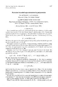
Fig. 16 共left兲 Final exterior mesh computed with the proposed technique. In total, 6,787 triangles were obtained after 31 digging iterations in 48 s. 共right兲 Adaptive triangular mesh obtained with Jade. Here 5,205 triangles were generated in 142 s.
optimization-free. For example, the 3D range image corresponding to the examples shown in Fig. 14 was approximated with the three methods using the same user-defined approximation error, = 0.041%. Jade generates a triangular mesh that approximates the 3D range image with 5,205 triangles. The result, in Fig. 16 共right兲, is slightly better than the one obtained with the proposed technique, in Fig. 16 共left兲, but Jade takes 142.7 s, while the proposed technique takes 48.84 s instead. The final exterior mesh obtained with the proposed technique contains 6,787 triangles. Simplification Envelopes is much more inefficient than Jade, since it generates a similar approximation with 5,495 triangles in 1,315 s. Note that although there is a small difference in the number of triangles contained in the final meshes, the most significant difference lies in the required CPU time. Therefore, the efficiency of the techniques in order to compute the required representations is used as the comparison criterion. In order to determine when a coarse-to-fine technique, such as the one proposed in this paper, is more advantageous than a fine-to-coarse approximation technique, such as Jade, the original 3D range image utilized in Fig. 14 was approximated with different adaptive triangular meshes corresponding to various tolerances, by applying both the proposed technique and Jade. It is assumed that both techniques generate similar results; hence, comparisons are based on CPU time. The geometry and number of triangles of the final meshes are similar in general, since, in all cases, they have to fit the original cloud of points according to the same user-defined approximation error. Figure 17 shows CPU times versus approximation errors for both algorithms. As expected, when an adaptive triangular mesh with a very low approximation error is required, the fine-to-coarse technique is much faster than the proposed technique. The reason is that the final exterior mesh is closer to the original dense mesh, which is the starting point of the fine-to-coarse algorithm. On the other hand, when a rather coarse adaptive triangular mesh is required, the proposed technique is more efficient than the fine-to-coarse approach; in this case, the solution is closer to the coarse mesh 共the convex hull兲 utilized as the starting point of the iterative digging process applied by the proposed technique. Hence, fewer iterations are necessary in order to reach the desired solution. Journal of Electronic Imaging
Fig. 17 Approximation error versus CPU time for the range image used in Fig. 14, by considering the proposed coarse-to-fine technique and a fine-to-coarse optimization technique 共Jade兲.
5 Conclusions and Further Improvements A new coarse-to-fine algorithm for generating boundederror triangular meshes from range images without optimization has been presented. This technique maps the pixels of a range image into a 3D curvature space. After tetrahedralizing those points with a 3D Delaunay algorithm, a digging process starts eroding the external surface of the resulting tetrahedralization until a mesh that fulfills the desired tolerance is obtained. The approximation error of that external surface is verified in the 3D image space. By avoiding iterative optimization stages, the proposed technique is advantageous with respect to previous coarseto-fine techniques based on iterative optimization, such as Refs. 17 and 22. Those techniques refine an initial triangular mesh of low resolution by adding one vertex at a time. At each iteration, the vertex that produces the highest reduction of approximation error must be found and inserted into the mesh, making them computationally intensive. Moreover, by working in a 3D curvature space, the proposed technique allows the adaptive approximation of both convex and nonconvex surfaces. This improves the behavior of previous coarse-to-fine sculpturing methods based on the 3D Delaunay triangulation, such as Refs. 20 and 24. By tetrahedralizing in the original 3D space instead of in the proposed curvature space, the latter methods approximate convex surfaces with the highest resolution, disregarding their curvature. Experimental results have shown that the proposed technique is more efficient than two well-known bounded-error simplification algorithms whenever a rather coarse resolution mesh is sought: a fine-to-coarse approach based on iterative optimization 共Jade21兲 and an optimization-free technique 共Simplification Envelopes19兲. Obviously, since the proposed iterative digging process starts refining the coarsest-resolution triangular mesh 共the convex hull兲, the proposed technique will require fewer iterations to reach a relatively coarse resolution mesh than iterative techniques that start with the highest-density triangular mesh and proceed by removing one point at a time.
023010-10
Apr–Jun 2007/Vol. 16(2)
Sappa and Garcia: Coarse-to-fine approximation of range images…
In general, coarse-to-fine approaches are more appropriate than fine-to-coarse ones for applications that require the generation of low-resolution representations that are subsequently refined only when necessary. This is a common procedure in order to accelerate a wide variety of algorithms in different fields, such as collision detection and path planning in robotics, scene visualization and ray tracing in computer graphics, or model-based image recognition in computer vision. As experimental results show, planar surfaces tend to be oversampled due to the presence of noise in the input range images, especially when low tolerances are specified. This undesired effect is likely to be reduced by applying discontinuity-preserving filtering techniques, such as in Ref. 27. Further work is necessary to evaluate the impact of these techniques on the whole approximation process. Acknowledgments This work has been partially supported by the Spanish Ministry of Education and Science under projects TRA200406702/AUT and DPI2004-07993-C03-03. The first author was supported by The Ramón y Cajal Program. References 1. P. Heckbert and M. Garland, “Survey of polygonal surface simplication algorithms,” in Multiresolution Surface Modeling Course, SIGGRAPH’97, Available online at ftp://ftp.cs.cmu.edu/afs/cs/project/ anim/ph/paper/multi97/release/heckbert/simp.pdf 共1997兲. 2. I. Cheng and P. Boulanger, “Feature extraction on 3D texmesh using scale-space analysis and perceptual evaluation,” IEEE Trans. Circuits Syst. Video Technol. 15共10兲, 1234–1244 共2005兲. 3. P. Csákány and A. Wallace, “Representation and classification of 3D objects,” IEEE Trans. Syst. Man Cybern. 33共4兲, 638–647 共2003兲. 4. K. Park, K. Lee, and U. Lee, “Models and algorithms for efficient multiresolution topology estimation of measured 3D range data,” IEEE Trans. Syst. Man Cybern. 33共4兲, 706–711 共2003兲. 5. Y. Sun, J. Paik, A. Koschan, D. Page, and M. Abidi, “Point fingerprint: A new 3D object representation scheme,” IEEE Trans. Syst. Man Cybern. 33共4兲, 712–717 共2003兲. 6. Z. Yan, S. Kumar, and J. Kuo, “Mesh segmentation schemes for error resilient coding of 3D graphic models,” IEEE Trans. Circuits Syst. Video Technol. 15共1兲, 138–144 共2005兲. 7. M. Andreetto, N. Brusco, and G. Cortelazzo, “Automatic 3D modeling of textured cultural heritage objects,” IEEE Trans. Image Process. 13共3兲, 354–369 共2004兲. 8. G. Guidi, J. Beralding, and C. Atzeni, “High-accuracy 3D modeling of cultural heritage: The digitizing of Donatello’s ‘Maddalena’,” IEEE Trans. Image Process. 13共3兲, 370–380 共2004兲. 9. R. Whitaker and E. Juarez-Valeds, “On the reconstruction of height functions and terrain maps from dense range data,” IEEE Trans. Image Process. 11共7兲, 704–716 共2002兲. 10. H. Hoppe, T. DeRose, T. Duchamp, J. McDonald, and W. Stuetzle, “Surface reconstruction from unorganized points,” Proc. SIGGRAPH’92, pp. 71–78 共1992兲. 11. M. Garland and P. Heckbert, “Surface simplification using quadric error metrics,” Proc. SIGGRAPH’97, pp. 209–216 共1997兲. 12. P. Lindstrom, “Out-of-core simplification of large polygonal models,” in Proc. SIGGRAPH’00, pp. 259–262 共2000兲. 13. Y. Zhu, “Uniform remeshing with an adaptive domain: A new scheme for view-dependent level-of-detail rendering of meshes,” IEEE Trans. Vis. Comput. Graph. 11共3兲, 306–316 共2005兲. 14. H. Hoppe, “Progressive meshes,” Proc. SIGGRAPH’96, 99–108 共1996兲.
Journal of Electronic Imaging
15. P. Lindstrom and G. Turk, “Evaluation of memoryless simplification,” IEEE Trans. Vis. Comput. Graph. 5共2兲, 98–115 共1999兲. 16. D. Brodsky and B. Watson, “Model simplification through refinement,” Proc. Graphics Interface, pp. 221–228 共2000兲. 17. L. De Floriani and E. Puppo, “Hierarchical triangulation for multiresolution surface description,” ACM Trans. Graphics 14共4兲, 363– 411 共1995兲. 18. M. Garcia and A. Sappa, “Efficient generation of discontinuitypreserving adaptive triangulations from range images,” IEEE Trans. Syst. Man Cybern. 34共5兲, 2003–2014 共2004兲. 19. J. Cohen et al., “Simplification envelopes,” Proc. SIGGRAPH’96, pp. 119–128 共1996兲. 20. L. De Floriani, P. Magillo, and E. Puppo, “On-line space sculpturing for 3d shape manipulation,” Proc. 15th IAPR Intl. Conf. Patt. Recog., pp 105–108 共2000兲. 21. A. Ciampalini, P. Cignoni, C. Montani, and R. Scopigno, “Multiresolution decimation based on global error,” The Visual Computer 13共5兲, 228–246 共1997兲. 22. L. De Floriani, “A pyramidal data structure for triangle-based surface description,” IEEE Comput. Graphics Appl. 9共2兲, 67–78 共1989兲. 23. C. Barber, D. Dobkin, and H. Huhdanpaa, “The Quickhull algorithm for convex hulls,” ACM Trans. Math. Softw. 22共4兲, 469–483 共1996兲. 24. J. Boissonnat, “Geometric structures for three-dimensional shape representation,” ACM Trans. Graphics 3共4兲, 266–286 共1984兲. 25. O. Faugeras, E. LeBras-Mehlman, and J. Boissonnat, “Representing stereo data with the Delaunay triangulation,” Artif. Intell. 44共2兲, 41–87 共1990兲. 26. OSU 共MSU/WSU兲, “Range image database,” available online at http://sampl.eng.ohiostate.edu/sampl/data/3DDB/RID/inddex.htm. 27. S. Li, “Highclose-form solution and parameter selection for convex minimization-based edge-preserving smoothing,” IEEE Trans. Pattern Anal. Mach. Intell. 20共9兲, 916–932 共1998兲. Angel D. Sappa received his electromechanical engineering degree in 1995 from National University of La Pampa, General Pico-La Pampa, Argentina, and his PhD degree in industrial engineering in 1999 from Polytechnic University of Catalonia, Barcelona, Spain. From 1999 to 2002 he undertook postdoctorate research at LAAS-CNRS, Toulouse, France, and at Z + F UK Ltd., Manchester, UK. From September 2002 to August 2003, he was with the Informatics and Telematics Institute, Thessaloniki, Greece, as a Marie Curie Research Fellow. Since September 2003 he has been with the Computer Vision Center, Barcelona, Spain, as a Ramón y Cajal Research Fellow. His research interests are focused on range image analysis, 3D modeling, and model-based segmentation. Miguel A. Garcia received his BS, MS, and PhD degrees in computer science from Polytechnic University of Catalonia, Barcelona, Spain, in 1989, 1991, and 1996, respectively. He joined the Department of Software at the Polytechnic University of Catalonia in 1996 as an assistant professor. In 1997 he joined the Department of Computer Science and Mathematics at, Rovira i Virgili University, Tarragona, Spain, as an associate professor, as head of Intelligent Robotics and Computer Vision Group. In 2006 he joined the Department of Informatics Engineering at Autonomous University of Madrid, where he is currently associate professor. His research interests include image processing, 3D modeling, and mobile robotics.
023010-11
Apr–Jun 2007/Vol. 16(2)