Minimum Error Bounded Efficient l1 Tracker with ... - Temple University

Minimum Error Bounded Efficient `1 Tracker with Occlusion Detection Xue Mei\ ∗ Haibin Ling† \ †

Yi Wu†[

Erik Blasch‡

Li Bai]

Assembly Test Technology Development, Intel Corporation, Chandler, AZ, USA

Center for Information Science & Technology, Computer & Information Science Department, Temple University, Philadelphia, PA, USA [

College of Computer and Software, Nanjing University of Information Science & Technology, Nanjing 210044, China ‡ ]

Air Force Research Lab/SNAA, OH, USA

Electrical and Computer Engineering Department, Temple University, Philadelphia, PA, USA

Abstract

tion changes. A thorough review can be found in [25]. Recently, sparse representation [5, 8] has been successfully applied to visual tracking [18, 15, 14]. In these methods, the tracking problem is formulated as finding a sparse representation of the target candidate using templates. The advantage of using the sparse representation lies in the robustness to a wide range of image corruptions, especially to an occlusion. The results show good performance, however, at a computational expense of the `1 minimization. Furthermore, the target states are estimated in a particle filter framework and the computational cost grows proportionally as the number of particle samples increases. The large computational cost prevents the tracker from being used in a real time system such as real time surveillance and military operations. Furthermore, the rich information captured in approximation coefficients has not been utilized for occlusion analysis. For example, a gradual occlusion may cause drifting in the template set. Inspired by the work mentioned above, we propose an efficient tracking algorithm with minimum error bound and occlusion detection. Our first contribution is to largely improve the run time efficiency of the L1 tracker by using an error bound derived from the least squares. Specifically, we observe that the computationally expensive reconstruction error in the sparsely constrained `1 minimization is lowerbounded by the least squares reconstruction error, which can be calculated efficiently. The reconstruction error observation motivates us to design a Bounded Particle Resampling (BPR) algorithm, which greatly boosts the speed of the tracking algorithm without sacrificing resampling precision. Specifically, the probability of tracking samples is calculated in two stages. In the first stage, the sample is reconstructed by simply projecting the sample onto the target template subspace. The reconstruction is solved through a linear least squares equation that runs several orders faster than a typical `1 minimization function. In the second stage, only dynamically selected samples that have smaller reconstruction errors from previous stage are reconstructed

Recently, sparse representation has been applied to visual tracking to find the target with the minimum reconstruction error from the target template subspace. Though effective, these L1 trackers require high computational costs due to numerous calculations for `1 minimization. In addition, the inherent occlusion insensitivity of the `1 minimization has not been fully utilized. In this paper, we propose an efficient L1 tracker with minimum error bound and occlusion detection which we call Bounded Particle Resampling (BPR)-L1 tracker. First, the minimum error bound is quickly calculated from a linear least squares equation, and serves as a guide for particle resampling in a particle filter framework. Without loss of precision during resampling, most insignificant samples are removed before solving the computationally expensive `1 minimization function. The BPR technique enables us to speed up the L1 tracker without sacrificing accuracy. Second, we perform occlusion detection by investigating the trivial coefficients in the `1 minimization. These coefficients, by design, contain rich information about image corruptions including occlusion. Detected occlusions enhance the template updates to effectively reduce the drifting problem. The proposed method shows good performance as compared with several state-of-the-art trackers on challenging benchmark sequences.

1. Introduction Visual tracking is an important topic for applications such as security and surveillance, vehicle navigation, human computer interaction, and so on. The challenges in designing a robust visual tracking algorithm in a dynamic environment are caused by the presence of noise, occlusion, varying viewpoints, background clutter and illumina∗ The work was done when Xue Mei was with University of Maryland, College Park.

1

through `1 minimization, while most of the samples are filtered out without solving the `1 minimization. By this two stage reconstruction, the computational cost is greatly reduced and the proposed tracker runs much faster than our previous L1 tracker [18]. Our second contribution is an occlusion detection method by investigating the reconstruction coefficients. It is then used to improve the template update procedure. The `1 minimization based reconstruction used in previous method [18] is known to be capable for capturing occlusion information, which has been previously used for face recognition [22]. While this property enables tracking occluded targets, it also induces risks by introducing the occluded target information into the template set and potentially causing track failures. To prevent the wrong information from contaminating the template set, we introduce a robust occlusion detection method. The idea is to first build an occlusion map from the trivial coefficients, which indicate pixel-wise image contamination in a given candidate. The occlusion map is then used for occlusion detection and a candidate is not added to the template set if an occlusion is detected. For evaluation, the proposed BPR-L1 tracker is tested on several challenging benchmark sequences involving challenges such as occlusion and illumination changes. In all the experiments, our BPR-L1 method shows excellent performance in comparison with previously proposed trackers.

2. Related Work Due to the extensive literature on visual tracking, we review only typical works and refer interested readers to [25] for a thorough review. The visual tracking problem can be formulated in two different categories: generative and discriminative. Generative tracking methods use an appearance model to represent the target observations. Tracking is formulated as searching the target location that has the most similar appearance to the model. Examples of generative tracking methods are eigentracker [3], mean shift tracker [7], incremental tracker [20], and covariance tracker [19]. In [20], a tracking method is presented that incrementally learns a low-dimensional subspace representation, and efficiently adapts to online changes in the target appearance. To adapt to the target appearance variations due to the illumination changes, pose changes, etc., the appearance model is often dynamically updated. Discriminative tracking methods cast the tracking as a binary classification problem. Tracking is formulated as finding the target location that can best separate the target from the background. In [1], a feature vector is constructed for every pixel in the reference image and an adaptive ensemble of classifiers is trained to separate pixels that belong to the object from pixels that belong to the background. In [6], a confidence map is built by finding the most discriminative RGB color combination in each frame. A hybrid

approach that combines a generative model and a discriminative classifier is used to capture appearance changes and allow reacquisition of an object after total occlusion [27]. Online multiple instance learning is used in [2] to achieve robustness to occlusions as well as other image corruptions. Global mode seeking is used to detect the object after total occlusion and reinitialize the local tracker [26]. Another example [4] uses image fusion to determine the best appearance model for discrimination and then a generative approach for dynamic target updates. Particle filter (PF) has been introduced for visual tracking [10] and has been a popular framework due to excellent performance for nonlinear target motion and flexibility to different object representations. While the use of more particle samples can improve track robustness, the computational load required by the particle filter also increases. Some authors have proposed to speed up the particle filter framework. In [24], the observation likelihood based on multiple features is computed in a coarse-to-fine manner so that the computation can quickly focus on the more promising regions. In [11], an efficient method is introduced for using subspace representations in a particle filter by applying Rao-Blackwellization to integrate out the subspace coefficients in the state vector. Fewer samples are needed since part of the posterior over the state vector is analytically calculated. In [28], it adjusts the number of particle samples based on the noise variance. Sparse representation has recently been introduced for tracking in [18] and later exploited in [15]. In [18], a tracking candidate is sparsely represented as a linear combination of target templates and trivial templates that only have one nonzero element in each of them. The sparse representation problem is solved through an `1 minimization problem with non-negativity constraints to solve the inverse intensity pattern problem during tracking. In [15] the group sparsity is integrated and very high dimensional image features are used for improving tracking robustness. Our work is inspired by these studies, but we use an `2 error bound to improve efficiency and introduce an occlusion map for reliable template updating. Our work shares philosophies with works where the error bound is used to guide visual tracking. For example, in [16] a boosting error bound in a co-training framework is used to guide the novel tracker construction. However, the application of using an error bound in a sparse tracker has not been well explored. Furthermore, our goal is to use the error bound for speed up without sacrificing accuracy.

3. Efficient L1-Tracker with Bounded Particle Resampling In this section we will first review the original L1Tracker [18] that combines the sparse representation and

the particle filter framework. Then we will present the least squares based minimum error bound, which can be more efficiently computed than the error bound used in the L1Tracker. After that, we propose the BPR-L1, using the BPR procedure to increase efficiency without accuracy loss.

3.1. L1-Tracker with Sparse Representation Particle filter. The L1-Tracker proposed in [18] is formulated as finding a sparse representation in the template subspace. The representation is then used with the particle filter framework [10] for visual tracking. Specifically, for frame at time t, we denote xt as the state variable describing the location and shape of a target. The tracking problem can be formulated as an estimation of the state probability p(xt |z1:t ), where z1:t = {z1 , z2 , · · · , zt } represents the observations from previous t frames. The tracking proceeds using a two-stage Bayesian sequential estimation, which recursively updates the filtering distribution as Z p(xt |z1:t−1 ) = p(xt |xt−1 )p(xt−1 |z1:t−1 )dxt−1 , (1) p(xt |z1:t ) ∝ p(zt |xt )p(xt |z1:t−1 ) ,

(2)

where p(xt |xt−1 ) indicates the state transition probability, and p(zt |xt ) gives the observation likelihood of state xt . Direct calculation of the above distribution is practically intractable. Alternatively, the posterior p(xt |z1:t ) is approximated by a set of N particle samples {xit }N i=1 with importance weights πti . The samples are updated and resampled at each frame. In the L1-Tracker, the state variable xt contains six parameters of the affine transformation. The state transition of xt are modeled independently by a Gaussian distribution around the previous state xt−1 , and N candidate samples are generated based on the state transition model p(xt |xt−1 ). The observation model p(zt |xt ) reflects the similarity between a target candidate and the target templates, which is formulated using approximation error in the sparse representation described as below. Sparse representation. To model the observation likelihood p(zt |xt ), a patch corresponding to state xt is first cropped from frame zt 1 . The patch is then normalized and reshaped to a 1D vector y, which is used as a target candidate. The sparse representation of y is formulated as a minimum error reconstruction through a regularized `1 minimization function with nonnegativity constraints min k Bc − y k22 +λ k c k1 , s.t. c < 0 , (3) c £ ¤ where B = T, I, −I is composed of target template set T and trivial template sets I and −I. Each column in T is a target template generated by reshaping pixels of a candidate 1 The

frame at time t is treated as the observation zt .

Algorithm 1 Particle filter for L1-Tracker 1: At t = 0, initialize samples xi0 , for i = 1, 2, · · · , N 2: for t = 1 to number of frames do 3: for i = 1 to number of samples do 4: Draw sample xit with respect to p(xt |xt−1 ) 5: Prepare the observation yit from xit . 6: Calculate the observation probability p(yit |xit ). 7: Resample with respect to p(yit |xit ), the number of times that xit appears in the new set is N ∗p(yit |xit ). 8: end for 9: end for patch into a column vector; and each column in the trivial template sets is a unit vector that has only one nonzero el£ ¤> ement. c = a> , e> is composed of target coefficients a and trivial coefficients e respectively. Finally, the observation likelihood is derived from the reconstruction error of y as 1 exp{−α k Ta − y k2 } , (4) Γ where a is obtained by solving the `1 minimization (3), α is a constant controlling the shape of the Gaussian kernel, and Γ is a normalization factor. For tracking at time t, the candidate with the maximum observation likelihood is chosen as the tracking result. The likelihood also serves for sample weights and resampling in the particle filter. A summary of the particle filter for L1Tracker is given in Algorithm 1. p(zt |xt ) =

3.2. Minimum Error Bound In this section, we will show that the reconstruction error from the target templates in `2 norm is bounded by a minimum error that can be calculated much faster than solving an `1 minimization function. Least squares error bound. The observation likelihood defined in (4) builds on the reconstruction error k Ta − y k2 measured in the `2 norm. Since a is calculated by the `1 minimization (3), there is a natural lower bound for the reconstruction error k Ta − y k2 ≥k Tˆa − y k2 ,

(5)

ˆa = arg min k Tb − y k2

(6)

where b

is the linear least approximation of y in the subspace spanned by T. One can also view ˆa as a degenerated case of a when λ = 0. Similarly, for the observation likelihood p(zt |xt ), we derive its upper bound q(zt |xt ) using the least squares approximation error q(zt |xt ) =

1 exp{−α k Tˆa − y k2 } , Γ

(7)

where α and Γ are the same as in (4). We immediately have p(zt |xt ) ≤ q(zt |xt ) .

(8)

Efficiency analysis. The linear system in (6) can be solved by Cholesky factorization or QR factorization. For dense matrices, the cost of the Cholesky factorization method is dn2 + (1/3)n3 , while the cost of the QR factorization method is 2dn2 , where d is the image dimension and n is the number of templates. The QR factorization method is slower by a factor of at most 2 if d À n, which is the case for our problem. For small and medium-size problems, the factor of two does not outweigh the difference in accuracy, and the QR factorization is the recommended method. The original L1-Tracker uses the preconditioned conjugate gradients (PCG) method [12] to solve the `1 minimization function. The PCG algorithm computes the search direction and the run time is determined by the product of the total number of PCG steps required over all iterations and the cost of a PCG step. The total number of PCG iterations required by the truncated Newton interior-point method depends on the value of the regularization parameter λ. In the experiments, we found that the total number of PCG is a few hundred. The computationally most expensive operation for a PCG step is a matrix-vector product which has O(d(2d + n)) = O(d2 + dn) computing complexity. From the complexity analysis, we can see the solution to the least squares problem in (6) is two orders faster than the `1 solution. For example, if we are using template size of 15 × 12, then d = 15 × 12 = 180. The number of templates is n = 10. The cost of Cholesky factorization method is dn2 + (1/3)n3 = 180 × 100 + (1/3) × 1000 ≈ 18000. While the cost of a PCG step is O(d2 + dn) = O(32400), and there will be a few hundred such steps.

3.3. Bounded Particle Resampling From the previous section, we showed that the computation is much more intensive to compute the observation likelihood p(zt |xt ) than to compute its upper bound q(zt |xt ). It is therefore attractive to use the upper bound for samples that are not promising enough and only conduct the true likelihood computations for the promising samples. In addition, to search for the candidate with the maximum likelihood, we still need the sample observations for resampling. Fortunately, in many cases only a small portion of the samples will be preserved after resampling and an efficient algorithm can be designed to avoid computing all observation likelihoods. We denote Xt = {x1t , x2t , · · · , xN t } as the sample set at time t, and denote pi = p(zt |xit ), qi = q(zt |xit ) as the observation likelihood and its corresponding upper bound defined in previous subsection. At the end of each frame, the samples are resampled with respect to their observation likelihoods. We have the following observation.

Algorithm 2 Two-stage Bounded Resampling 1: 2: 3: 4: 5: 6: 7: 8: 9: 10: 11: 12: 13: 14: 15: 16: 17: 18: 19: 20: 21:

Input: sample set Xt−1 = {xkt−1 }N k=1 Output: sample set Xt = {xkt }N k=1 /*Stage 1*/ for i = 1 to N do Draw sample xit from xit−1 Prepare the sample appearance yit from xit Solve the linear least squares problem (6) for yit Compute qi according to (7) end for Sort samples in descending order according to qi /*Stage 2*/ i ← 1, τ1 ← 0 while qi ≥ τi and i ≤ N do Solve the `1 minimization problem (3) for yit Compute pi according to (4) τi+1 ← τi + pi /(2N − 1) i←i+1 end while pj ← 0, ∀j ≥ i /*Resampling*/ N Xt ← Resample {xkt }N k=1 with respect to {pk }k=1

Observation 1. If the sample appears at least once in the resampled set, its observation probability must satisfy the following condition N

1 X pj . (9) 2N j=1 The observation is straightforward because the number of samples remains unchanged before and after resampling. The “2” in the denominator is due to rounding. Motivated by the observation, we develop a two-stage bounded resampling algorithm to calculate the probability of the tracking candidates. The first stage is very straightforward: we compute the probability bounds qi for all samples and sort them in descending order. Without loss of generality, in the following we assume the samples are already sorted, i.e., q1 ≥ q2 ≥ · · · ≥ qN . In the second stage, our task is to calculate the observation probability pi for samples that will survive resampling. The observation probability can be done efficiently even for large number of samples by using a dynamically updated threshold τ to exclude to-be-discarded samples. In particular, τ is defined according to the following theorem: pi ≥

Theorem 1. If the ith sample xi appears at least once after resampling, its likelihood bound qi is no less than a threshold τi defined as i−1

X 1 τi = pj . 2N − 1 j=1

(10)

Proof. From Observation 1, we have pj ≥

j=1

i X

pj .

j=1

Subtract pi on both sides and divide by 2N − 1, we have pi ≥

1 2N − 1

i−1 X

pj = τi .

(12)

log(p) log(q) log(τ)

−10

(11) probability

2N pi ≥

N X

0

−20

−30

−40

j=1

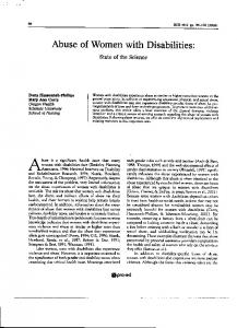
Using the fact that qi is an upper bound of pi , we have qi ≥ pi ≥ τi . From the definition, we see that the thresholds are nondecreasing, i.e., 0 = τ1 ≤ τ2 ≤ · · · ≤ τN , and there is pi τi+1 = τi + , (13) 2N − 1 which can be used for an efficient threshold update. With the above thresholds, in the second stage we start with the first sample that has the largest likelihood bound q1 , and calculate the probability p1 according to (4) and update the corresponding threshold τ2 according to (13). Then we continue for samples 2, 3, . . .. For the ith sample, if the likelihood bound qi ≥ τi , we compute the observation likelihood pi and update threshold τi+1 . Otherwise if qi < τi , which according to Theorem 1 implies that xi , xi+1 , · · · , xN will be discarded during resampling. Then, we directly set pi = pi+1 = · · · = pN = 0. The probabilities p1 , p2 , · · · , pN is then used for resampling set X . The proposed two stage bounded resampling is summarized in Algorithm 2. The above Bounded Particle Resampling (BPR) procedure does not sacrifice resampling precision, which is guaranteed by Theorem 1. BPR avoids the expensive computation on samples with low likelihoods. The amount of time saved is mainly determined by the dissimilarity between the tracking foreground and its surrounding background. Intuitively, the larger the foreground/background difference, the more speedup from the BPR procedure. Furthermore, the BPR framework encourages using more particles with larger sampling variance in comparison with the previously proposed L1-Tracker [18]. BPR helps improve tracking accuracy in addition to computational efficiency. Empirical studies. In Fig. 1, it shows the curves of p, q, and τ calculated from one frame when 600 particles are used. After about 100 particle samples, q is becoming smaller than τ , and the probability p of the rest samples are assigned to 0 without calculating the computational expensive `1 minimization. For this frame, only 20% of the samples need to solve the `1 minimization, and we achieve about 5 times speed up for this frame. Fig. 2 shows the run time and the number of particle samples for which the `1 minimization is performed. We can see that the run time is proportional to the number of the

−50 0

100

200 300 400 particle sample

500

600

Figure 1. The curves of p, q, and τ . The logarithm is applied to the data for display purpose.

Figure 2. The run time and number of particle samples for sequence OneLeaveShopReenter2cor.

samples and is dominated by the second stage probability calculation. For most of the frames in the sequence, only 20% of the particle samples calculate the `1 minimization. From frame 190 to 230, the man comes out of the shop and the woman is partially occluded. We clearly see that the number of particles calculating for the `1 minimization increases dramatically when the target is occluded. When the target is occluded, none of the samples can model the target appearance well enough so the probabilities are distributed between the particles. The more probabilities concentrate on the first few samples, the less particles are needed for the `1 minimization calculation. When the probabilities are evenly distributed, more particles are needed, which results in a longer run time for the frame.

4. Occlusion Detection The template set needs to be updated to capture the appearance variations of the target during tracking. In [18], the tracking result is added to the template set if none of the template is similar to the tracking result. Therefore, the tracker is vulnerable to failures when the tracking re-

sult with a large occlusion is added to the template set. To prevent an improper addition to the template set, we propose a method to detect the large occlusion in the tracking result before it is added to the template set. For occlusion detection, we investigate the responses in the trivial templates when solving the `1 minimization (3). The trivial templates are activated when the pixel intensity can not be approximated well using the target templates. Therefore, we explore the trivial template coefficients for the occlusion detection. We convert the 1D trivial coefficient vector to a 2D trivial image by reversing the way that the target template is vectorized. Each pixel in trivial image is mapped to the pixel in the same location in the template image. We threshold the trivial image and obtain another 2D binary image that we call occlusion map. The white pixel in the occlusion map indicates that the pixel is occluded and the black pixel indicates no occlusion. We assume that an occluder is large in size and the intensity is different enough to be separated from small random noises. Therefore, the occlusion is a large connected region in the occlusion map. The occlusion detection is then reduced to find a white area that is large enough to be classified as an occlusion. After applying morphological operations to the occlusion map to remove the small areas and fill the small hole between the regions, we count the number of pixels in the largest region. If the area is larger than a pre-defined threshold, say 30% of the area of the occlusion map, we conclude that there is an occlusion in the tracking result, and the template set should not be updated. Normally when an occlusion is detected, it will not go away for a certain period of time. For example, when the target is occluded by an object, and the object is moving away from the target, the occlusion is becoming smaller before it goes away. In our occlusion detection method, we avoid updating the template set for the next 5 frames after an occlusion is detected.

5. Experiments We implemented the proposed approach in MATLAB with the SPAM package2 [17]and evaluated the performance on seven publicly available video sequences.3 Our proposed tracker is compared with seven latest state-ofthe-art trackers named Incremental Visual Tracking (IVT) [20], Multiple Instance Learning (MIL) [2], Visual Tracking Decomposition (VTD) [13], Generalized Kernel Tracking (GKT) [21], L1 tracker (L1) [18], Covariance Tensor Learning (CTL) [23], and Online AdaBoost (OAB) [9]. The 2 http://www.di.ens.fr/willow/SPAMS/downloads.html 3 Sequences 1–3 were from http://www.cs.toronto.edu/˜dross/ivt/. Sequences 4–7 were from the PETS 2001 dataset http://www.cvg.cs.rdg.ac.uk/ PETS2001/, http://groups.inf.ed.ac.uk/vision /CAVIAR/CAVIARDATA1/, http://vision.stanford.edu/˜birch/headtracker /seq/, and http://vision.ucsd.edu/˜bbabenko/project miltrack.shtml.

tracking results of the compared methods were obtained by running the source code or binaries provided by their authors using the same initial positions in the first frame.

5.1. Qualitative Comparison The first sequence shows a vehicle undergoes drastic illumination changes as it passes beneath a bridge and under trees. Tracking results on several frames are presented in Fig. 3 (A). The BPR-L1 tracker, L1 tracker, IVT and CTL are able to track the target well even though the drastic illumination changes, while the other trackers lose the target after it goes through the bridge. The second sequence was captured in an indoor environment. Results on several frames are presented in Fig. 3 (B). The BPR-L1 tracker, L1 tracker, IVT, OAB, and MIL tracks the target faithfully throughout the sequences. The other trackers fails track the target when there are both pose and illumination changes. Results on the third sequence are shown in Fig. 3 (C). It shows a moving animal doll and presents challenging pose, lighting, and scale changes. The L1 tracker, IVT, and VTD eventually fails in frame 736 as a result of a combination of drastic pose and illumination change. The BPR-L1 tracker and rest trackers are able to track the target for this long sequence, though GKT is a little off the target in frames 521, and 546. In the fourth sequence, a person is walking from right bottom corner to the left of the image (Fig. 3 (D)). The IVT fails to track the target from the start. The VTD starts to show some target drifting around 200 frames, and finally loses the target. Our tracker and the rest trackers successfully track the target. The fifth sequence is to track a walking woman. In this video, the background color is similar to the color of the woman’s trousers, and the man’s shirt and pants have a similar color to the woman’s coat. In addition, the woman undergoes partial occlusion. Some result frames are given in Fig. 3 (E). Only the BPR-L1 tracker and L1 tracker are able to track the target during the entire sequence. The other trackers lock on the man when he occludes the woman after he comes out of the shop. Results of the sixth sequence are shown in Fig. 3 (F). In this sequence, we show the robustness of our algorithm in handling occlusion and large pose change. All the trackers track the target in the entire sequence except for the MIL that loses the target in the frame 466. Results on the seventh sequence are shown in Fig. 3 (G). Many trackers start drifting from the target when the man’s face is almost fully occluded by the book. The BPR-L1 tracker handles this very well and continues tracking the target when the occlusion disappears.

(A) Car4 (23, 185, 210, 271, 306, 599) #0023

#0185

#0210

#0271

#0306

#0599

(B) David Indoor (318, 411, 442, 463, 595, 677) #0318

#0411

#0442

#0463

#0595

#0677

(C) Sylvester (28, 238, 365, 521, 546, 736)

(D) PETS01D1Human1 (1417, 1496, 1562, 1631, 1744, 1821)

#0028

#0238

#0365

#1417

#1496

#1562

#0521

#0546

#0736

#1631

#1744

#1821

(E) OneLeaveShopReenter2cor (6, 193, 205, 244, 325, 467)

(F) Girl (30, 107, 247, 332, 439, 466)

#0006

#0193

#0205

#0030

#0107

#0247

#0244

#0325

#0467

#0332

#0439

#0466

(G) Occluded Face 2 (43, 152, 354, 473, 706, 786) #0043

#0152

GKD

#0354

MIL

OAB2 1 0

#0473

CTL

#0706

VTD

IVT

#0786

L1

Our tracker

Figure 3. Tracking results of different algorithms. Frame numbers are listed after sequence names.

5.2. Quantitative Comparison To quantitatively compare robustness under challenging conditions, we manually labeled the ground truth of the seven sequences. The tracking error evaluation is based on the relative position errors (in pixels) between the center of the tracking result and that of the ground truth. Ideally, the position differences should be around zero. As shown in Fig. 4, the position difference results of the BPR-L1 tracker are much smaller than those of the other trackers. Using the BPR method, the BPR-L1 tracker accounted for occlusion errors and better utilized particle re-

sampling for computational efficiency and track accuracy.

6. Conclusion We propose an efficient BPR-L1 tracker with minimum error bound and occlusion detection. We employ a twostage sample probability scheme, where most samples with small probabilities from first stage are filtered out without solving the computational expensive `1 minimization. Our occlusion detection coupled with a template update scheme effectively prevents the tracking result with a heavy occlusion from adding that tracking result to the target template

200

100

150

100

Sylvester 160

GKD MIL OAB CTL VTD IVT L1 Our tracker

140 Position Error (pixel)

300

Position Error (pixel)

Position Error (pixel)

400

David Indoor 200

GKD MIL OAB CTL VTD IVT L1 Our tracker

50

120 100 80

PETS01D1Human1 700

GKD MIL OAB CTL VTD IVT L1 Our tracker

600

Position Error (pixel)

Car4 500

60 40

200

300 400 Frame #

500

600

100

OneLeaveShopReenter2cor

Position Error (pixel)

100 80 60

400

100

200

Girl

40

100

300 200

300

400 500 Frame #

600

700

800

600

700

800

0

100

200 Frame #

300

400

Occluded Face 2

150

GKD MIL OAB CTL VTD IVT L1 Our tracker

Position Error (pixel)

120

200 300 Frame #

0

200 GKD MIL OAB CTL VTD IVT L1 Our tracker

Position Error (pixel)

100

0

400

100

20 0

500

GKD MIL OAB CTL VTD IVT L1 Our tracker

50

150

100

GKD MIL OAB CTL VTD IVT L1 Our tracker

50

20 0 0

100

200 300 Frame #

400

500

0

100

200 300 Frame #

400

500

0

100

200

300

400 500 Frame #

Figure 4. Quantitative comparison of the trackers in terms of position errors (in pixel).

set. Preventing an incorrect update to the target template set reduces track failure. Our proposed BPR-L1 method is computational more efficient than the previous L1 trackers, and demonstrates the effectiveness in handling a number of challenging sequences. We compared the BPR-L1 tracker with seven other state-of-the-art trackers including the original L1 tracker on seven sequences to validate robustness. Acknowledgment This work is supported in part by NSF Grants IIS-0916624 and IIS-1049032. Wu is supported in part by NSFC (Grant No. 61005027).

References [1] S. Avidan. “Ensemble Tracking”, CVPR, 494-501, 2005. 2 [2] B. Babenko, M. Yang, and S. Belongie. “Visual Tracking with Online Multiple Instance Learning”, CVPR, 2009. 2, 6 [3] M. J. Black and A. D. Jepson. “Eigentracking: Robust matching and tracking of articulated objects using a view-based representation”, IJCV, 26:63-84, 1998. 2 [4] E. Blasch and B. Kahler. “Multiresolution EO/IR Target Tracking and Identification”, Int. Conf. on Info Fusion, 2005. 2 [5] E. Cand`es, J. Romberg, and T. Tao. “Stable signal recovery from incomplete and inaccurate measurements”, Comm. on Pure and Applied Math, 59(8):1207-1223, 2006. 1 [6] R. T. Collins, and Y. Liu. “On-Line Selection of Discriminative Tracking Features”, ICCV, 346-352, 2003. 2 [7] D. Comaniciu, and V. Ramesh, and P. Meer. “Kernel-based object tracking”, IEEE PAMI, 25:564-577, 2003. 2 [8] D. Donoho. “Compressed Sensing”, IEEE Trans. Inf. Theory, 52(4):1289-1306, 2006. 1 [9] H. Grabner, M. Grabner, and H. Bischof. “Real-time tracking via online boosting”. BMVC, 4756, 2006. 6 [10] M. Isard and A. Blake. “Condensation - conditional density propagation for visual tracking”, IJCV, 29:5-28, 1998. 2, 3 [11] Z. Khan, T. Balch, and F. Dellaert. “A Rao-Blackwellized particle filter for EigenTracking”, CVPR, 980-986, 2004. 2 [12] S.-J. Kim, K. Koh, M. Lustig, S. Boyd, and D. Gorinevsky. “A method for large-scale `1 -regularized least squares”, IEEE J. on Sel. Topics in Signal Processing, 1(4):606-617, 2007. 4

[13] J. Kwon and K. M. Lee. “Visual Tracking Decomposition”, CVPR, 1269-1276, 2010. 6 [14] H. Ling, L. Bai, E. Blasch, and X. Mei. “Robust Infrared Vehicle Tracking across Target Pose Change using L1 Regularization,” Int. Conf. on Info Fusion, 2010. 1 [15] B. Liu, L. Yang, J. Huang, P. Meer, L. Gong, and C. Kulikowski. “Robust and Fast Collaborative Tracking with Two Stage Sparse Optimization”, ECCV, 2010. 1, 2 [16] R. Liu, and J. Cheng, and H. Lu, “A robust boosting tracker with minimum error bound in a co-training framework”, ICCV, 2009. 2 [17] J. Mairal, F. Bach, J. Ponce and G. Sapiro. “Online Learning for Matrix Factorization and Sparse Coding.” JMLR, 11:19–60, 2010. 6 [18] X. Mei and H. Ling. “Robust Visual Tracking using `1 Minimization”, ICCV, 2009. 1, 2, 3, 5, 6 [19] F. Porikli, O. Tuzel and P. Meer. “Covariance tracking using model update based on lie algebra”, CVPR, 728-735, 2006. 2 [20] D. Ross, J. Lim, R. Lin and M. Yang. “Incremental learning for robust visual tracking”, IJCV, 77:125-141,2008. 2, 6 [21] C. Shen, J. Kim and H. Wang. “Generalized Kernel-based Visual Tracking”, TCSVT, 20(1), 119-130, 2010. 6 [22] J. Wright, A. Y. Yang, A. Ganesh, S. S. Sastry, and Y. Ma. “Robust Face Recognition via Sparse Representation”, IEEE PAMI, 31(1):210-227, 2009. 2 [23] Y. Wu, J. Cheng, J. Wang, and H. Lu. “Real-time Visual Tracking via Incremental Covariance Tensor Learning”, ICCV, 2009. 6 [24] C. Yang, R. Duraiswami, and L. Davis. “Fast multiple object tracking via a hierarchical particle filter”, ICCV, 2005. 2 [25] A. Yilmaz, O. Javed, and M. Shah. ‘Object tracking: A survey”. ACM Comput. Survey, 38(4), 2006. 1, 2 [26] Z. Yin and R. Collins. “Object tracking and detection after occlusion via numerical hybrid local and global mode-seeking”, CVPR, 2008. 2 [27] Q. Yu, T. B. Dinh and G. Medioni. “Online tracking and reacquistion using co-trained generative and discriminative trackers”, ECCV, 2008. 2 [28] S. K. Zhou, R. Chellappa, and B. Moghaddam. “Visual tracking and recognition using appearance-adaptive models in particle filters”, TIP, 11:1491-1506, 2004. 2