applications presented are a seesaw/pendulum process and aerodynamics of a ... Performance will be the issue in the seesaw/pendulum example below while ...
Code Generation for Simulation and Control Applications (IMS99).nb
1
Code Generation for Simulation and Control Applications Mats Jirstrand and Johan Gunnarsson MathCore AB
Mjärdevi Science Park SE-583 30 Linköping Sweden Third International Mathematica Symposium 1999, 23-25 August, RISC, Linz, Austria
Abstract The use of Mathematica in combination with MathCode C++ is illustrated in a context of modeling of dynamical systems and design of controllers. The symbolic tools are used to derive a set of nonlinear differential equations using Euler-Lagrange equations of motion. The model is converted to C++ using MathCode C++, which produces an efficient implementation of the large expressions used in the model. The exported code is used for simulations, which illustrates that Mathematica in combination with MathCode C++ can be used to do accurate and powerful simulations of nonlinear systems. Controller synthesis is performed where the resulting controller is exported to C++ and run externally. The applications presented are a seesaw/pendulum process and aerodynamics of a fighter aircraft.
1 Introduction Control system design is a discipline where advanced mathematics is applied to real world problems ranging from paper and pulp manufacturing, aircraft, and CD players to bio-chemical processes, logistics, and financial applications. Mathematica is very powerful for dealing with the mathematics in these control problems and the application package Control System Professional (CSP) implements many useful features. When it comes to nonlinear systems the combination of the symbolic and numeric capabilities of Mathematica makes modeling and control system design in this environment very attractive. The notebook concept for documentation of different trade-offs and decisions during the design process also contributes to making Mathematica suitable for this kind of work. The application package MathCode C++ adds automatic C++ code generation to Mathematica, which can be used both to enhance performance of simulations of large systems and to generate stand-alone C++ code to be used in applications separately from Mathematica. Performance will be the issue in the seesaw/pendulum example below while the standalone feature is explored in the fighter aircraft example. The stand-alone code generation feature of MathCode C++ makes it possible to design and prototype a controller in Mathematica and then "lift out" the resulting stand-alone code
Code Generation for Simulation and Control Applications (IMS99).nb
2
to be used in the real control system. This minimizes the need of coding the control law manually from the algorithms designed in Mathematica. In this document we will try to illustrate the use of Mathematica together with MathCode C++ for modeling, control system design, and code generation. The document is organized as follows. In the rest of this section we give some basic facts about dynamic systems needed to formulate controller design problems. In Section 2 a nonlinear mechanical system is modeled and simulated using generated C++ code. In Section 3 controller design for an aircraft is done and in Section 4 we give some conclusions.
à Preliminaries Many dynamic systems can be modeled by a set of first order differential equations, see e.g. [1, 2] dx@tD
€€€€€€€€ dt € € = f@x@tD, u@tDD y @tD = g @x@tDD
(1)
where f : Ñn ‰ Ñm ® Ñn . Here x@tD Î Ñn , u@tD Î Ñm, and y@tD Î Ñ p are called the states, inputs, and outputs of the system, respectively. Equation (1) is called the state space form of the equations describing the behavior of the system and is particularly useful for control system design. We will also use the dot-notation x for denoting differentiation w.r.t. time dx
€€€€dt€€€ . If the system is linear the state space form can be written as dx@tD
€€€€€€€€ dt € € = A .x@tD + B.u@tD, y @tD = C.x@tD
(2)
where A Î Ñn‰n , B Î Ñn‰m, and C Î Ñ p‰n are constant real matrices. If f @0, 0D = 0 in (1) the system can be linearized around x=0, u=0. The A, B, and C matrices are then computed from f and g by taking partial derivatives as follows A = €€€€€€€€ ¶x€ €€€€€€ É x=0 , ¶f@x,uD
É x=0 , u=0
B =
¶f@x,uD €€€€€€€€ ¶u€ €€€€€€
(3)
C = €€€€€€€€ ¶x € € É x=0
u=0
¶g@xD
The linearized model is usually a good approximation whenever the states and input to the system are small. There exists a large number of control design methods for linear systems which makes it desirable to work with linear models if possible during controller synthesis. The performance of the resulting controller can then be studied in simulations where the linear model has been exchanged with the nonlinear one. A linear state-feedback controller is a very simple type of controller where the control signal is a linear combination of the states that are assumed to be measurable. Hence, a linear state-feedback law has the form u[t] = -L.x[t]
(4)
There exists many methods for computing the matrix L but a necessary condition is that the chosen L makes the closed loop system asymptotically stable, which essentially means that non-zero states converge to zero. More or less advanced methods makes it possible to compute L such that different trade offs between performance and robustness can be obtained, see e.g. [1, 4, 5]. A slightly more advanced controller is the linear dynamic controller, which includes an internal model of the system to be controlled. A so called observer is used to estimated the states x@tD of the system from measured signals y@tD and a linear
Code Generation for Simulation and Control Applications (IMS99).nb
3
feedback law is used to compute the input to the system to be controlled. Using the notation x` @tD for estimated states the linear dynamic controller can be written as follows d` x@tD ` €€€€€€€€ dt € €€€ = A c .x @tD + B c .y@tD, ` u@tD = - L.x @tD
(5)
Hence, a dynamic controller requires real time solving of a system of differential equations. In the seesaw/pendulum example below we will use a linear state-feedback controller of the form (1) and in the fighter aircraft example we will use the observer based controller of the form (5).
2 The Seesaw/Pendulum Process In this section we will illustrate how the symbolic capabilities of Mathematica can be used to derive a model of a nonlinear system. Using MathCode C++ the large symbolic expressions in the nonlinear model are then converted to C++ code and used to simulate the system very efficiently. The system is a laboratory process frequently used in control education known as the seesaw/pendulum process. One implementation of the seesaw/pendulum process has been developed by Quanser Consulting (http://www.quanser.com).
à The System The process consists of a seesaw, two carts called C1 and C2 , two parallel tracks, an inverted pendulum, and a weight. Each cart can be driven by a DC motor controlled by an input voltage. Cart C1 carries the weight and cart C2 carries the inverted pendulum attached by a friction free joint. The carts can be moved along the tracks by controlling the input voltages of the DC motors. We start by modeling the open loop system, i.e., without any feedback from measured signals. The forces F1 and F2 acting on each cart are chosen as inputs. We will use the Lagrangian methodology to obtain a nonlinear model of the system and then linearize it. The linearized model is used for control system design where the Control System Professional (CSP) application package is used. The closed loop system are then simulated both within Mathematica and by external code generated using MathCode C++.
Code Generation for Simulation and Control Applications (IMS99).nb
Figure 1. The Pendulum/Seesaw Process.
In Figure 1 we introduce names of variables and constants describing the process. Variables: x1 x2 q a F1 F2
translation of cart 1 from center of track translation of cart 2 from center of track angle of seesaw with vertical angle of inverted pendulum with normal to track force applied to cart 1 force applied to cart 2
Constants: J ms c h m1 m2 mp lp g
inertia of seesaw with track at height h mass of seesaw with track height of center of gravity of the seesaw from pivot point height of track from pivot point mass of cart 1 (weight cart, on the back track) mass of cart 2 (pendulum cart, on the front track) mass of pendulum center of mass of pendulum rod (half of full length) gravitational acceleration
The physical values of the above constants are stored as rules in Mathematica to be used later on in simulations. physicalvalues := 9 J ® 1.6, ms ® 6.6, c ® 0.06, h ® 0.115, 0.61 m1 ® 0.48 + 0.38, m2 ® 0.48, mp ® 0.2, lp ® €€€€€€€€€€€€€ + 0.03, g ® 9.81= 2
4
Code Generation for Simulation and Control Applications (IMS99).nb
5
à Modeling Following the Lagrangian methodology [3] the system is divided in a number of subsystems whose potential energy and kinetic energy are computed in terms of the generalized coordinates introduced in Figure 1 above. The Lagrangian, which is the difference between the total kinetic and potential energy, can then be used to derive the equations of motion for the system. Ÿ Computation of the Lagrangian Coordinates of the center of mass of the seesaw
xs := c Sin@q@tDD ys := c Cos@q@tDD The potential and kinetic energies of the seesaw
Vs := ms g ys
1 Ts := SimplifyA €€€€€ J H¶t q@tDL2 E 2 Coordinates of the center of track
xc := h Sin@q@tDD yc := h Cos@q@tDD Coordinates of cart 1 x m1 := xc + x1 @tD Cos@q@tDD y m1 := yc - x1 @tD Sin@q@tDD The potential and kinetic energies of cart 1
V m1 := m1 g y m1
1 T m1 := SimplifyA €€€€€ m1 HH¶t x m1L2 + H¶t y m1L2 LE 2 Coordinates of cart 2 x m2 := xc + x2 @tD Cos@q@tDD y m2 := yc - x2 @tD Sin@q@tDD The potential and kinetic energies of cart 2
Code Generation for Simulation and Control Applications (IMS99).nb
V m2 := m2 g y m2
1 T m2 := SimplifyA €€€€€ m2 HH¶t x m2L2 + H¶t y m2L2 LE 2 Coordinates of the center of mass of the pendulum
xp := x m2 + lp Sin@a@tD + q@tDD yp := y m2 + lp Cos@a@tD + q@tDD The potential and kinetic energies of the pendulum
Vp := mp g yp
1 Tp := SimplifyA €€€€€ mp HH¶t xp L2 + H¶t ypL2 LE 2 The total potential energy
Vtot := Vs + V m1 + V m2 + Vp The total kinetic energy
Ttot := Ts + T m1 + T m2 + Tp The Lagrangian of the system
L := Ttot - Vtot The Lagrangian of the system becomes
6
Code Generation for Simulation and Control Applications (IMS99).nb
7
Simplify@LD 1 €€€€€ I-2 c g Cos@q@tDD ms - 2 g m1 Hh Cos@q@tDD - Sin@q@tDD x1 @tDL 2 2 g m2 Hh Cos@q@tDD - Sin@q@tDD x2@tDL -
2 g mp Hh Cos@q@tDD + Cos@a@tD + q@tDD lp - Sin@q@tDD x2 @tDL + J q¢@tD2 + m1 IHh2 + x1@tD2 L q¢@tD2 + 2 h q¢@tD x¢1 @tD + x¢1 @tD2M + m2 IHh2 + x2 @tD2L q¢ @tD2 + 2 h q¢@tD x¢2 @tD + x¢2@tD2 M + mp HHHh Cos@q@tDD - Sin@q@tDD x2@tDL q¢ @tD +
Cos@a@tD + q@tDD lp Ha¢@tD + q¢@tDL + Cos@q@tDD x¢2 @tDL ^ 2 +
HHh Sin@q@tDD + Cos@q@tDD x2 @tDL q¢ @tD + Sin@a@tD + q@tDD lp Ha¢ @tD + q¢@tDL + Sin@q@tDD x¢2 @tDL^ 2LM
Ÿ Computation of the Equations of Motion The equations of motion are given by the partial differential equations that L must satisfy d ¶L ¶L €€€€ €€ €€€€€€€ - €€€€ €€ Š Qi, i = 1, ¼ , n , dt ¶q ¶qi
(6)
i
where L is the Lagrangian, q i , i = 1, ¼, n are the generalized coordinates, and Qi , i = 1, ¼, n are the generalized force associated with each coordinate. In this case the quadruple 8q 1 , q 2, q 3 , q 4< corresponds to 8x1, x2 , q, a< and Q1 = F1 , Q2 = F2, Q3 = Q4 = 0. We derive each equation and simplify it eqn1 = Simplify@¶t H¶¶t x1@tD LL - ¶x1@tD L == F1 D; eqn2 = Simplify@¶t H¶¶t x2@tD LL - ¶x2@tD L == F2 D; eqn3 = Simplify@¶t H¶¶t q@tD LL - ¶q@tD L == 0D; eqn4 = Simplify@¶t H¶¶t a@tD LL - ¶a@tD L == 0D; These equations are coupled ordinary differential equations (ODEs) of second order in the generalized coordinates x1 , q, x2 , a. To rewrite these in standard state space form (a system of first order ODEs) we introduce the following states: x = H x1 q x2 a x1 q x2 a L.
The inputs to the system are u = H F1 F2 L.
We observe that the second order time derivatives of the positions and angles appears linearly which makes it easy to solve for these in terms the states. Second order time derivatives will always appear linearly in the equations derived from the partial differential equation (6) that the Lagrangian of the system has to satisfy. This is due to the fact that the Lagrangian only consists of at most first order time derivatives and the second order derivatives appear according to the ¶L chain rule when differentiating the term €€€€ €€€€€ in (6) w.r.t. time. ¶q i
Solve for second order derivatives
Code Generation for Simulation and Control Applications (IMS99).nb
8
sol = Solve@ 8 eqn1 , eqn2 , eqn3, eqn4