CodeCloud: A Platform to Enable Execution of Programming Models on the Clouds Miguel Caballera,∗, Carlos de Alfonsoa , Germ´an Molt´oa , Eloy Romeroa , Ignacio Blanquera , Andr´es Garc´ıaa a Instituto
de Instrumentaci´ on para Imagen Molecular (I3M). Centro mixto CSIC – Universitat Polit` ecnica de Val` encia – CIEMAT, camino de Vera s/n, 46022 Valencia, Espa˜ na
Abstract This paper presents a platform that supports the execution of scientific applications covering different programming models (such as Master/Slave, Parallel/MPI, MapReduce and Workflows) on Cloud infrastructures. The platform includes i) a high-level declarative language to express the requirements of the applications featuring software customization at runtime; ii) an approach based on virtual containers to encapsulate the logic of the different programming models; iii) an infrastructure manager to interact with different IaaS backends; iv) a configuration software to dynamically configure the provisioned resources and v) a catalog and repository of virtual machine images. By using this platform, an application developer can adapt, deploy and execute parallel applications agnostic to the cloud backend. Keywords: Cloud computing, Virtual Infrastructures, Elasticity, Contextualization
1. Introduction Scientific computing has long been devoted to close the gap between scientists, who require executing resource-starved models, and computer scientists, who can deliver the power required to solve challenging computational problems. In the last decades, different computing infrastructures have been used to provide computing power to the scientific community. Moreover with the commoditization of hardware, clusters of PCs became a suitable platform for scientists to execute their workloads. However, scientific problems required computational resources far beyond the capacity of a single cluster of PCs. The increase in network bandwidth made utility computing possible. Organizations started sharing computational power and storage (among other resources) in the so-called Grids, where scientific users could execute large experiments. Grid computing has proved to be a valuable tool not only to foster collaboration among research but also to aggregate enough computing power to tackle challenging problems that could not have been solved before [1]. ∗ Corresponding
author Email address:
[email protected] (Miguel Caballer)
Preprint submitted to Elsevier
February 20, 2014
However, the Grid also exposed some drawbacks for scientists, since they had to adapt their applications to fit the requirements of the underlying computing platforms (in terms of Operating System, software libraries, etc.). Although the Scientific Gateways made progresses towards abstracting the usage of the Grid [2], the diversity of platforms and software configurations made the approach a compile-once run-anywhere difficult. This hindered the massive adoption of the Grid out of the academic environment, which typically remained composed by Virtual Organizations with pre-configured environments and tools. With the advent of Cloud Computing, the idea of utility computing is reconsidered. The use of virtualization and its ability to customize the underlying infrastructure to the requirements of the applications (not the other way round, as in Grid computing) opened new opportunities. Cloud computing enabled users to migrate clustered based applications to cloud-computing resources without modifying the existing resources. The usage of virtualized infrastructures on top of Cloud infrastructures enables to dynamically deploy suitable computing platforms, such as a virtual cluster. In this way users are provided with larger computing capabilities, but with the software and environment they are familiar. Therefore scientists can run their unmodified codes on modern computer resources without investing time in porting their applications to new computer designs. For that, this paper describes an architecture and the implemented platform (called CodeCloud) to perform the execution of scientific applications on Cloud computing infrastructures, supporting different programming models (currently Master/Slave, Parallel/MPI, Workflow and MapReduce). The scientists just need to provide a high-level description of the jobs to be executed, the programming model required, and the computing and execution environment requirements. Then, the system performs the automatic provision of the virtual infrastructure that satisfies the aforementioned requirements, executes and monitors the jobs, including data management. The platform features both horizontal and vertical elasticity capabilities to dynamically allocate and deallocate resources from both on-premise Clouds (such as OpenNebula and OpenStack) and public Cloud providers (including Amazon Web Services). This paves the way for scientists to easily access vast computing resources on-demand with minimal investment in application porting. After the introduction, the remainder of the paper is structured as follows. First, section 2 describes the related work in this area. Next, section 3 provides a high-level overview of the CodeCloud architecture and its components. Then, section 4 describes the CJDL domain specific language that enables the user to define the jobs to be executed providing a common abstraction layer that insulates the user from knowing the internal details of the Cloud deployment. Later, section 5 defines the architecture and details the software components developed, it also shows the elasticity capabilities of the platform. Section 6 describes a study case to demonstrate the functionality of the developed platform. Finally section 7 summarises the paper and points to future work. 2. Related Works The execution of scientific applications on the Cloud involves i) the provision of Cloud computing resources, mainly computational nodes and storage; ii) the deployment of the applications and their dependent services; and iii) the dynamic adaptation of the resources provisioned to the variable requirements of the applications at runtime. 2
Most of these aspects are shared by applications that successfully migrated to the Cloud or those that were developed for the Cloud leaning their developments on some PaaS (Platform as a Service, [3]). A PaaS solution creates an environment for developers to access Cloud resources from a high-level perspective, without dealing with the infrastructure details. The developer is provided with an API (or SDK) to compose the services offered by the platform but no direct interaction with the infrastructure (the Virtual Machines) is performed. Therefore, an abstraction for the execution of services and applications is provided. 2.1. Platform as a Service Solutions There are some well-known commercial PaaS solutions such as Google App Engine (GAE) [4], Microsoft Azure [5] and Amazon Web Services (AWS) [6]. They provide support for their own commercial Cloud infrastructures and services allowing the development of applications in several languages like .NET, Java or Python. Another commercial solution is PaaS Manjrasoft Aneka [7], a software platform that provides a runtime environment and a set of APIs that allow developers to build .NET applications that leverage their computation on either public or private Clouds. Aneka provides special support to coordinated tasks (using a similar interface to the one used for programming threads) and Map/Reduce operations. There also exist free PaaS platforms. For example, Heroku [8] can deploy applications using a large set of languages and environments such as Ruby, Node.js, Clojure, Java, Python, and Scala. It also provides a large set of third party services like databases, caching, monitoring, performance management, etc. to enhance the applications. CloudFoundry [9] supports the application development frameworks Spring, Ruby on Rails, Ruby and Sinatra, Node.js and Grails. It also provides a set of services to the application developers such as some relational database management systems (i.e., MySQL, PostgreSQL), Redis for a key-value NoSQL database and RabbitMQ as a messaging service. AppScale [10] is an open source implementation of the GAE PaaS Cloud technology. As a new development over AppScale, Neptune [11] is a domain specific language over Ruby that automates the configuration and deployment on multiple nodes of applications based on MPI or Hadoop MapReduce. Besides its simple user interface, it is noteworthy the support for launching on multiple IaaS at the same time and recycling unused nodes in order to reduce the final per-hour cost. However, like the rest, it does not enable to customize the VMs with user requirements. ConPaaS [12] is a runtime environment to run applications in the Cloud supporting OpenNebula and Amazon EC2 Cloud deployments. It currently includes a Web hosting service supporting PHP and Servlets, a MySQL database service, a batch processing service and a MapReduce service. In ConPaaS, an application is defined as a composition of one or more services. The availability of a custom budget-constrained scheduler for the batch processing service [13] is specially interesting. However, there are still details that remain unsolved. Scientific users do not have to deal with the set-up of their local environments. Clouds never require users to do so. In Table 1 the comparative between the mentioned platforms is extended considering aspects such as 1) the software license type; 2) the software interface of the product; 3
eC lo u C
od
S C on Pa a
ep tu ne N
A
ne ka
d
Table 1: Comparison among several platforms similar to CodeCloud. Abbreviations: CF, configuration files; WUI, web user interface accessed through a web browser; Automat. VMI intrument., automatic VMI instrumentation; Progr., programming. † Will soon be available for download with GPL license.
No SDK/GUI
Yes SDK
Yes WUI
Yes† CF
3) Public IaaS support 4) Custom VMI 5) Automat. VMI instrument. 6) Basic Orchestration
Yes Yes No No
Yes No – No
Yes Yes Yes No
Yes Yes Yes Yes
7) Elasticity 8) Cost optimizer 9) QoS/SLA support
Yes Yes Yes
Yes Yes No
Yes Yes Yes
Yes No No
No Yes Yes Yes Custom Progr. Yes
Yes Progr. Yes No Yes No Partial
Yes Basic No No No No No
Yes Yes Yes Yes Yes Yes Yes
Yes Yes
No Yes
No Yes
No No
1) Open source 2) Software interface
10) Command-line executions 11) Parameter Sweeping 12) MPI 13) Master-Slave 14) MapReduce 15) Workflow 16) Data Management 17) Licensing Management 18) Users Management
4
3) the capability of provisioning from public IaaS; 4) whether a custom VMI can be used to deploy the VMs and 5) in that case if a configuration is required previously; 6) if an automatic management of applications is supported; 7) if rules can be defined to dynamically resize the provisioned resources, and 8) if it is done considering heuristics to minimize the final cost and 9) the fulfillment of Quality of Service (QoS) and Service Level Agreement (SLA) specifications; 10–15) the programming models supported; 16) if some abstraction is offered to identify and move files using different protocols; and 17) if there is some support to control the use of the resources by applications and 18) users. 2.2. Related Tools for Cloud Computing In addition to the aforementioned approaches, which completely manage the lifecycle of application execution in the Cloud, many tools have been developed only focused on specific steps in this lifecycle. For example, in Cloud resources provisioning there are tools like boto1 or AWS to access the Amazon Web Services, and other IaaS agnostic like DeltaCloud2 , Libcloud3 and fog4 . In addition, Nimbus [14] is an open source IaaS system offering EC2, S3 and WSRF interface. It also provides tools to automate the deployment and configuration of a virtual cluster [15], and to manage the elasticity [16]. Other tools focus on automating the installation, configuration and contextualization of applications, sometimes referred as orchestration. The installation and part of the configuration are usually carried out by installing packages available on software repositories, such as those provided by each GNU/Linux distribution, or associated to specific programming languages. In complex deployments, the orchestration tools can group the different software configurations by roles, and provide means for the nodes with the same role to exchange information together enabling the aggregation of information from other roles. Ansible5 , Puppet6 and Chef7 are examples of software with the aforementioned capabilities. After the development and configuration of the infrastructure and services for an application, the next step is to perform the execution of the application. For this purpose, 1 http://boto.readthedocs.org/en/latest 2 http://deltacloud.apache.org/about.html 3 http://libcloud.apache.org/about.html 4 http://fog.io 5 http://ansible.cc 6 http://www.puppetlabs.com 7 http://www.opscode.com/chef
5
SAGA Pig
SLA & Elasticity ConPaaS
Neptune Aneka
MapReduce Pegasus Swift HTCondor Task SGE PBS/Torque Declaration
CodeCloud Nimbus
DeltaCloud fog Libcloud
IaaS boto
Infrastructure Deployment Orchestration
Ansible Juju Puppet Chef
AWS
Figure 1: Conceptual map grouping the main specific tools and PaaS solutions in scientific cloud computing by its functionality.
it is important to understand the parallel model of the applications. For example, High Throughput Computing (HTC) applications are composed by a large number of tasks with weak dependencies which involve intense computational resources or data processing. This applications typically use a scheduler, such as PBS/Torque, HTCondor or SGE, to distribute the workload among the available computing resources. Compatibility among different schedulers is supported either by allowing the scheduler to relaunch to other batch systems (e.g., HTCondor can talk to other schedulers like PBS/Torque), and also by the schedulers understanding other job APIs. For the latter, there are two notable examples, Simple API for Grid Applications (SAGA) [17] (being saga-python [18, 19] one of its major implementations) and Distributed Resource Management Application API (DRMAA) [20] (implemented by most of the schedulers). The MapReduce programming model has been intensively used in Cloud computing, being Apache Hadoop the free source reference implementation. It receives important criticism (the challenge of its deployment, its dependence on HDFS distributed filesystem and its rigid model that makes difficult the execution of multiple operations) that has motivated the development of several alternatives, such as Pig, Twister (both allowing several MapReduce jobs), Sector/Sphere [21] (based on stream processing [22] instead of file chunks) and SAGA based (focusing on decoupling the task management from the data sources). Another hot topic in computing science is workflow modeling. Workflows define complex control and data dependences among the different tasks of an application. It is difficult to find a single API specification or implementation as reference for workflows [23]. Some of them need a scheduler as a backend, like Pegasus that uses HTCondor through the DAGman interface. Finally, as Fig. 1 depicts, the most specific tools (around the corners) cover the declaration of tasks, and the provision (tagged as IaaS ) and configuration of resources (Orchestration), while the dynamic adaptation to the application requirements (SLA & Elasticity) is found integrated in many of the mentioned PaaS solutions for scientific 6
computing, as shown on Table 1. Most of Cloud developments (IaaS, PaaS and others) rely on existing tools, instead of developing new ones. The efficient management of scientific applications execution lies at the intersection of the technologies that enable infrastructure provisioning and automated application deployment together with SLA-based execution management and the ability to leverage the elasticity of the Cloud platforms. These are precisely the core functionalities available in the CodeCloud platform, described in the following section. 3. The CodeCloud Architecture This section describes the CodeCloud architecture. It provides a high-level overview of the platform, along with its main capabilities. The following sections will cover the implementation aspects of the principal components of CodeCloud. The proposed approach uses the concept of container, similar to the approach used by Web Services containers such as Apache Tomcat, in which a (WAR) file is employed to provide the description and functionality of the service. Once deployed, the Web Service is ready to be accessed. In CodeCloud, the container encapsulates not only the programming model logic but also all the infrastructure needed to execute it in the cloud. Each application launched has its own container that manages the whole life-cycle of the cloud execution (avoiding some multi-tenancy problems such as security or accounting). In the proposed approach, an Enhanced Virtual Container (EVC) consists of a Virtual Machine (VM), which encapsulates i) a virtual hardware configuration, in terms of CPU architecture, disk size, RAM, ii) an Operating System (OS), and iii) a set of libraries and software where a specific service, developed to process the applications of one of the programming models, is deployed. The Enhanced Virtual Container (EVC) provides the following features: • Infrastructure management: The EVC provisions the virtual infrastructure with specific hardware features. • Contextualization: It enables the infrastructure to be configured with the software to support both the programming model and the user application at runtime. • Monitoring: An agent collects monitoring information of the state of all the virtual infrastructure created, including the EVC itself (CPU load, disk usage, etc.) and the state of the running application. • Elasticity: It manages both the horizontal (scale in / out) and vertical (scale up / down) elasticity. • Data management: The EVC will download into the infrastructure all the input data needed to execute the application prior the its execution. It will also upload the output data to the data storage endpoint provided by the user. • Execution: The EVC enables the user application to be launched in the virtual infrastructure specifically created and customized with the precise requirements of the application. 7
VMRC
Inf. Manager
3. Create Prog. Model Container
7. Launch the Inf. 6. Create Inf. for the App
CJDL
1. Launch Cloud App.
4. Launch VM and contextualize the Container
CodeCloud Service
VM (Worker) Prog. VMModel (Worker) Prog. VMModel (Worker) Prog. Model
CJDL
2. Return Job ID 5. Launch Job
...
Manage the Job status Monitor
Container VM Prog. Model (Puppet Master)
8. Configure Inf
9. Start execution
Upload Input Data (optional) Cloud Data Service (CDMI)
VM (Worker) Prog. Model VM (Master) Prog. Model
Upload Output Data (Optional)
Figure 2: Architecture of the CodeCloud platform.
Figure 2 summarises the architecture of the proposed system. The user submits to the CodeCloud Service (CCS) a description of the jobs to be executed on a Cloud infrastructure. For that, it has been defined the Cloud Job Definition Language (CJDL), a high-level declarative language (described later on). This document includes the definition of the jobs, which can refer to external resources (input data files, executable files, etc.) in a remote server. Before submitting a job, the client has to upload the input local files (for instance, to a Cloud storage service that supports the CDMI interface [24]) and refer the files by their corresponding URLs. The CJDL document includes a section described using the Resource Application Description Language (RADL) [25]. The RADL is a is a declarative language for the end-users to describe the computational infrastructure needed to run their applications, by declaring the features or requisites of the VMs to be deployed. When the user submits an application execution request (step 1), the user receives an identifier that can be used to follow the execution progress of the jobs. Both the CCS and EVC need to provision the virtual infrastructure required to execute the jobs. For that, it relies on the Infrastructure Manager (IM) [25], which takes as input the RADL section of the CJDL document. The IM in turn queries a catalog of VMIs called Virtual Machine image Repository and Catalog (VMRC) [26], which indexes VMIs together with metadata concerning the features of each VMI (SO, installed applications, etc.). This enables the IM to choose the most appropriate VMI to deploy the virtual infrastructure. Back to Figure 2, the CCS contacts the Infrastructure Manager (IM) to create a VM where the programming model’s EVC chosen by the user will be deployed (step 3). The 8
container will be in charge of deploying and managing the infrastructure requested by the user and the subsequent submission and monitoring of the jobs. Once the EVC is up and running, the CCS submits the CJDL document to the EVC so that job submissions can be started (step 5). From now on, the container takes control of the submission process. First of all, it verifies the RADL document specified in the CJDL. Each programming model should take the RADL given by the user to ensure that the created VMs will satisfy its requirements, not only the ones imposed by the user but also the hardware and software requirements necessary for the programming model to operate. For example in the case of the MapReduce model a Hadoop cluster will be installed and configured and in the case of Master/Slave, MPI and Workflow models a Torque/PBS cluster will be installed. This way, the IM deploys the VMs with all the required features to properly function (step 6). Once all the nodes are up and running, the programming model’s container configures all the infrastructure nodes to make the programming model to work. For that purpose, Puppet has been used to push the configuration and the software required to setup the nodes according to the user’s requirements. Puppet has a widespread usage and an active community. It can describe high-level recipes using a declarative domainspecific language. An specialization for the EVC has been created for each programming model, even though all of them have a common interface and share similar functionality. Each programming model just customizes certain parts of the EVC. Then, the infrastructure is ready to submit the application jobs for the specified programming model. Therefore, the EVC contacts the main node of the infrastructure, copies all the required files and submits the jobs (step 9). The execution step depends on the programming model selected. For example, in the case of MapReduce, a corresponding job will be submitted to the configured Hadoop cluster. In the other models, the EVC will create a set of Torque tasks performing the necessary job submission operations to the underlying LRMS (Local Resource Management System). During the execution, the EVC monitors the state of the application to notify the CodeCloud service about the execution process. But the EVC also monitors the infrastructure state (CPU, RAM, disk, etc.) using Ganglia [27], which is installed and configured in all the nodes in the contextualization step. When the execution finishes, the container must copy the output data files to the specified destination in the CJDL. Finally, it stops and releases all the VMs deployed. The last step consists on releasing the VM of the container. In this case, the CCS is responsible for ensuring that all data have already been staged out in order to destroy the EVC. 4. CJDL: Cloud Job Description Language This section describes the Cloud Job Description Language (CJDL), a domain specific language that aims at simplifying the task of migrating already existing applications to Cloud environments. This declarative language provides a common abstraction layer that frees the user from the need to understand the internal details of the Cloud deployment. This language has been inspired by the Job Description Language (JDL) [28], widely used to define Grid jobs and based on Condor classads. As opposed to JDL, CJDL is formated in XML to gain in readability (by humans and machines) and ease its processing. 9
Different programming models are supported by CJDL to ease the expression of the functionality and requirements of user’s applications. The most popular parallel programming models have been considered, to cover a wide range of applications used by the scientific community: • MapReduce [29]. MapReduce is a programming model typically used for processing and generating large datasets. Users specify the main computation in terms of a map and a reduce function, and the underlying runtime system automatically parallelizes the computation across large-scale clusters of machines sharing a distributed file system. A static specification is made of the problem partitioning, the unit of work, the scheduling and the merging of results. • Master/Slave [30]. This programming model is used when the number of jobs is higher than the number of resources, and a master process dispatches the jobs to the slave (working) nodes. The partitioning in this case can be dynamic and reconfigured either by the application or by the resource manager. • Workflow [31]. This programming model is composed by a sequence of connected steps (tasks to be performed). The execution order of the tasks is different if the workflow is data-driven (in which the output data of a task represents the input data of another task), or task-oriented workflow (in which a child task is only executed when the parent task has finished). This model describes the different processing units, the input and output data and the execution arguments. The parallelism is defined by the data and the processes. • Parallel/MPI [32]. This programming model performs parallel executions based on the Message Passing Interface (MPI) on a cluster of PCs with distributed memory. The scientific community is using a large amount of legacy MPI applications which efficiently solve, in terms of computational power and memory consumption, different scientific problems. A CJDL document comprises several parts that define the requirements in terms of resources, software dependencies and programming models. Next subsections describe these parts and the relation to the mentioned programming models. 4.1. Infrastructure Description The tag Infrastructure contains the information concerning the Cloud infrastructure that needs to be deployed to execute the application. The section includes VM descriptions in RADL language of the infrastructure requirements in terms of number and type of machines, its features (CPU, RAM, disk, etc.), operating system and preinstalled software, among other. Networking features can also be specified. 4.2. Programming Model Roles Under the tag Configuration it is specified a mapping between the VMs defined in the RADL (the type attribute) and the roles in the programming model (the name attribute). In addition, the initial, minimum and maximum number of instances that are submitted for every type of machine are indicated by the attributes count, min and max respectively. All the programming models have a node that manages the execution 10
of the tasks (named Main) and other that performs the execution of the tasks (named Worker). The next example corresponds to a MapReduce deployment in which the frontend (the role Main) will run on a VM described as front in the RADL, and that can scale out up to one more node; and the tasks will be run initially on four and up to 20 VMs (the role Worker) described as wn in the RADL: 4.3. Execution Description Under the tag ExecutionData the tasks that compound the cloud job are listed. The task include descriptions of the details in the deployment (i.e., the needed files and where are stored), the launching (i.e., the environment and the command line template) and the dependencies to other tasks. This part is where the programming models show their differences and where it is more challenging to express all the programming models supported in an easy and consistent manner. Our approach is based on the workflow engine WINGS [33]. At first glance, WINGS is a data-driven workflow: Jobs in WINGS are executed when data defined as input is available in the data source and write the result in other data source defined as output. If the input tag contains files from a data source, the engine will copy the files to some local place before launching the job, injecting the location of the file as a commandline argument. In cases such as MapReduce (which use legacy applications), the executions have specific names (partitioner, mapper and reducer) and the engine transfers the input files to (and back at the end from) the Hadoop Distributed File System. A complete example of MapReduce is presented in Figure 3. The data sources are very abstract bags of data, ranging from read-only list of values, to a collection of files. The files can be available locally to the machine that is launching the cloud job (indicated by the URI lfile) or be local to the machine that is running the job (indicated by file) or can be stored remotely in a server that supports for instance FTP, SFTP or CDMI: 11
Under the activity tag the inputs of a job are defined as they will appear in the commandline, including the deployment details. Most of the software and hardware requirements are specified in the RADL section, so only the specification of the executable and additional files to be downloaded in run-time (and if using MPI, the minimum and maximum number of nodes that can be used) are described here. If the mpi attribute is set to yes, the application will be launched in parallel with “mpiexec”. Similarly in the MapReduce model a jar file and a class can be specified as executable for native Hadoop applications instead of using the partitioner, mapper and reducer executions. The WINGS engine was extended to deal with dependency cycles of jobs and data sources. This feature is used for instance in some Master/Slave applications whose master dynamically launches new jobs after processing the result of previous ones (if it is not the case, the application can be modelled as simple workflows). Moreover in generic (non Hadoop) map-reduce applications, reduction jobs need to has the output data source also as an input one. Besides, WINGS was modified in order to support task-driven workflows like pure Directed Acyclic Graph (DAG) workflows. Therefore a new section is included to indicate the relations among the different tasks defined in the execution section: 4.4. Elasticity The tag Configuration contains the initial, minimum and maximum number of instances that are submitted for every type of machine (with the features specified in the RADL document) to deploy the initial infrastructure. But if the application requirements change, the platform must have the ability to adapt the resources to the application load using a set of elasticity rules. The elasticity section enables the user to specify the rules that define the elasticity modes of the infrastructure during the execution of the application. An elasticity rule has the following syntax:
if then [for ] 12
• Rule: The rule specifies, considering the monitoring information of either the infrastructure or the application, the condition that will trigger the action to modify the features of the infrastructure. The metric used in the rules are expressed using a declarative language using similar concepts to those shown in RADL, such as cpu.usage or memory.free. In addition, other general concepts concerning the execution can be employed, such as app.pct finish or execution.time. Also, other values concerning each programming model can also be used, such as app.tasks queued, in the case of Master/Slave. Finally, the user can also utilize application-dependent values by properly modifying the application to use the container API to publish the state update of such values, as shown later. It must be considered that the EVC stores historic values for each metric. So the general concept metrics will refer an array of n elements (with n as the number historic elements stored) and the VM related values will be a matrix with n · v elements (with v as the number of VMs in the infrastructure). So it is required for a set of functions to reduce these set of values to a single one to use them in the comparative operations. First three operations are used to reduce the set of values in one dimension: min, max and avg. As the VM values are matrices, two operations will be needed to obtain a single value. Also an operator {} enables selecting the last num historic elements. If this operator is not included all the stored values will be used. Finally, an operator [] enables filtering a set of values of an specified VM type. • Action: The action that will be performed to modify the infrastructure. There are four functions: two provides the horizontal elasticity and other two for the vertical one: – ScaleIn/ScaleOut: Remove/Add resources to the infrastructure. This function receives two parameters: the type and number of resources to add/remove. The type of resources is a string value that refers a system name defined in the RADL code in the Infrastructure section of the CJDL document (e.g. node in the CJDL example in Figure 3). – ScaleUp/ScaleDown: Increase/Decrease the capacities of a set of VMs of the infrastructure. This receives as parameters the type of resource to modify (cpu or memory) and the amount of resources to modify. • Filter: This last parameter is optional, it is used only in the case of vertical elasticity operations, and it enables to select a subset of VMs to apply the corrective action. The syntax used is the same used in the specification of the rules. Here we show several examples of elasticity rules. In the first three examples the ScaleIn/ScaleOut are used to provide horizontal elasticity. In the last two, the functions ScaleUp/ScaleDown are used to provide vertical elasticity. • A rule to enable deploying a new VM if the CPU usage of the virtual infrastructure is high (over 90%). In particular, if the mean value (considering all the machines) of the average value of the CPU usage of each of the machines vmtype1 during the last 5 time periods is greater than 90%, the system should deploy 1 VM of type vmtype1 and 2 machines of type vmtype2. 13
if avg(avg(cpu.usage[vmtype1]{5})) gt 90% then ScaleIn([1,2], [vmtype1, vmtype2]) • A rule to enable deploying 2 new VMs if the free memory of the virtual infrastructure is low (lower than 50MB). In particular, if the average value of the minimum value of free memory of all the VMs during the last 2 periods of time is lower than 50 MB, It should deploy 2 machines of type vmtype1.
if avg(min(memory.free{2}) lt 50MB then ScaleOut(2, vmtype1) • A rule to enable undeploying 2 VMs application is progressing adequately. In particular if the application progress is over 80% and the execution time is lower than 5 minutes, then undeploy 2 VMs of type vmtype1.
if execution.pct_finsh gt 80% and execution.time lt 5:00 then ScaleIn(2, vmtype1) • A rule to enable increasing the memory in the VMs if the free memory is low (lower than 50MB). In particular, if the minimum value of the average value of the free memory of all the VMs during the last 5 periods of time is lower than 50 MB, then increase in 512 MB the memory of the VMs with the average value of the free memory during the last 5 periods of time that has been lower than 50 MB.
if min(avg(memory.free{5})) lt 50MB then ScaleUp(512M, memory) for avg(vm.memory.free{5}) lt 50MB • A rule to enable increasing the number of CPUs to the VMs with high CPU usage (over 90%). In particular, if the maximum value of the average value of the cpu usage of all the VMs during the last 4 periods of time is over 90%, add 1 CPU to the VMs with the average value of the CPU usage during the last 4 periods of time that is over 90%.
if max(avg(cpu.usage{4})) gt 90% then ScaleUp(1, cpu) for avg(vm.cpu.usage{4}) gt 90% Vertical elasticity must also be supported by the underlying hypervisor. In particular, in previous works we focused on dynamic memory management of VMs to fit the underlying virtual infrastructure to the dynamic memory consumption of scientific applications, using the KVM hypervisor [34]. 4.5. Example use case of CJDL A CJDL document corresponding to the MapReduce job of the BLAST application [35] that will be presented as test case next in section 6 is given in this part8 . In MapReduce, the definition of a task that uses legacy applications is provided by three parameters: i) the partitioning of the input data set, ii) the map function and iii) 8 Some
parts of the document has been omitted for the sake of clarity
14
system node ( cpu.count>=1 and cpu.arch=’x86_64’ and memory.size>=1024 and disk.0.os.flavour=’ubuntu’ and disk.0.os.version=’12.04’)
... ...
Figure 3: The CJDL for the MapReduce application in CodeCloud.
the reduce function, to join the output data files into a single final result. Then the execution of applications that follow this programming model requires: i) the execution of the data partitioning, ii) generating as many map tasks as parts of the initial data set and, once all the map tasks have finished, iii) performing the reduce task to join all the processed results in order to generate the output data. In the CJDL in Figure 3, the user defines the node type node with at least 1 GB of RAM on an Ubuntu 12.04 Linux system. Initially, one VM with the “Main” role in the MapReduce programming model and five nodes with the “Worker” role are requested. In the dataGroup “dc1” the user specifies the application input data, the “/data/blast” directory the machine that is launching the job is specified. Also the “/data/output” local directory is specified to store the final output data. Then, the activities referring the functionality of the partitioner, mapper and reducer operations are defined, operations that are finally called in the executions section.
15
5. Infrastructure Provision and Elasticity Management 5.1. Infrastructure Deployment The infrastructure has been deployed using previous developments covered in [25]. For the sake of completeness, a brief summary of each development is included here: • VMRC is a Virtual Machine Repository and Catalog system, which is used to find a suitable VMI that accomplishes the requirements of the user and it is compatible to the available cloud system. This component stores and indexes VMIs in order to be reused in multiple contexts. It also implements a matchmaking algorithm to obtain the VMIs that satisfy a set of requirements. • Infrastructure Manager: It is a system that orchestrates the different components, enabling the effective deployment of an initial computing infrastructure, and the further operations to modify it on demand, adding or removing virtual nodes. The IM exposes an API with a reduced and simple set of functions enabling the creation of the infrastructure, getting the information about the VMs, and adding or removing of VMs in the deployment. Using these components, the necessary steps to create the virtual infrastructure are summarized as follows. First, the requirements of the infrastructure (software and hardware) are described using RADL. Second, the IM contacts the VMRC to find the most appropriate VMI considering the requirements. Finally, the IM deploys an instance of the VMI in a Cloud backend (currently supports OpenNebula, OpenStack and Amazon EC2). 5.2. Elasticity One of the functionality that containers provide is the ability to export a structured NoSQL database based on key/value pairs to provide information about the application execution and about the infrastructure. Some of these data are the same for all the programming models, such as the information concerning the infrastructure: CPU usage, disk usage, etc., in addition to other general values regarding the execution (provided by the programming model container): percentage of finish, execution time, etc. However, each model can also export specific values to obtain more precise information. For example, in the case of Master/Slave, this information includes the total number of tasks, the number of active and finished tasks, etc. In the case of the Workflow programming model, the node in the workflow that is currently being executed. To gain extensibility, applications can also use an API to publish application-dependent specific values, such as the value of a variable in a given point in time. This would allow to better track the execution of an application and opens the way to enable computational steering in the Cloud, where an execution could possibly be cancelled if a given variable reaches a certain value. Figure 4 shows the inner work of the elasticity manager. The EVC relies on Ganglia to monitor the infrastructure nodes. Therefore, when contextualizing (configuring) the infrastructure, the Ganglia agent is installed in all the nodes and configured so that the Main node stores the aggregate information from all the nodes of the deployment for a given execution under a programming model. The EVC exposes all the information 16
VM Container SLA Monitor
Take Measures
Inf. Manager
Get Info
Catalog
Register SLAs
Push Information
Get Info
EVC
Ganglia
Add or Remove Nodes
API
Collect Inf. Information VM WN Ganglia
VM WN Ganglia
VM WN
...
Ganglia
Figure 4: Elasticity manager.
taken as input for the elasticity rules in the shape of key/value pairs. We consider both the information of the EVC itself (% of execution, execution time, etc.) and the metrics obtained with Ganglia (currently considering CPU usage, memory usage and disk usage). This information is exposed through the EVC’s API, which can also be employed for modified applications to publish their own data for it to be also considered for elasticity rules. All this information is periodically submitted to the catalog using its REST interface. The catalog stores the historical information. When the EVC starts, it must register the elasticity rules in the Monitor. The monitor periodically evaluates the rules by querying the historical information stored in the catalog taking the appropriate measures (horizontal or vertical scaling) by delegating on the IM. 6. Case Studies This section includes two case studies that exemplify the usage of the CodeCloud platform for the execution of scientific applications under different programming models. 6.1. MapReduce To demonstrate the functionality of the system the MapReduce example shown in the 4.5 section has been launched in the CodeCloud platform. The application launched is the High-Throughput version of BLAST. The experiment aligns the dataset of sequences of mammals from the UNIPROT protein database [36] (4MB) against sequences of invertebrates form the same database (555MB). This experiment may conclude the degree of transference of genes among the two zoological groups. BLAST is a tool that performs such alignment. A MapReduce approach to solve the BLAST problem is shown in Figure 3. In the partition step it is executed a “split.sh” script that divides the input file in FASTA format, into smaller pieces (the seqfile*.sqf files) that will be processed by the 17
Table 2: MapReduce use case times
Input Data Uploaded Container VM Prepared Infrastructure Launched Infrastructure Configured Total Deployment Execution Time Output Data Downloaded Total Time
1 node (ONE) 0:14 2:20 7:33 3:51 13:58 15:00:33 0:01 15:14:32
5 node (ONE) 0:13 2:21 10:57 7:12 20:43 3:10:55 0:01 3:31:39
10 node (ONE) 0:15 2:31 16:32 19:45 39:03 2:31:04 0:01 3:10:08
1 nodes (EC2) 10:07 1:50 4:01 7:02 23:00 36:25:10 0:08 36:48:18
5 nodes (EC2) 10:00 1:51 5:31 10:23 27:45 8:03:10 0:07 8:31:02
10 nodes (EC2) 9:02 1:51 7:32 15:39 34:04 6:12:10 0:07 6:46:21
mapper functions. The mapper operations executes the blast command with each partition. Finally the reducer combined all the output data from the mappers into a single file result. Both the input and output data are referenced using the special “lfile” scheme. So the CodeCloud client must initially upload the input data from the user’s machine and finally download the output data to it. The same case study has been executed on an on-premise OpenNebula deployment and on Amazon EC2 with 1, 5 and 10 nodes. In particular, the OpenNebula deployment used has been supported by four Dell Servers in Blade format (M600 and M610 models). Each server has eight cores and 16 Gb of RAM and are mounted on a M1000e chassis. In the Amazon EC2 case it has been used the “m1.small” instances (as it fulfils the user requirements of the RADL document) in the “us-east-1” region. The time needed to deploy the infrastructure can be decomposed into the following steps: • Input data uploaded: Time needed to upload the data to the cloud storage (560MB). The data are initially stored in the user’s machine and it must be uploaded to a cloud storage to be available to the container. In the case of the OpenNebula deployment the data and the cloud storage system are in the same local network and the transfer time is reduced. In the EC2 case the data must be uploaded to a cloud storage system located in the EC2 infrastructure so the time needed is considerably larger. • Container VM Prepared: Time spent to launch the container VM. In the OpenNebula case the time used in this step is mainly the transference of the VMI to the physical node where it will be deployed. The container VMI is about 3.5GB and the time needed is relatively small. In Amazon EC2 the container VMI uses an EBS-backed AMI (Amazon Machine Image) and the time needed to launch this kind of VMIs is very small. • Infrastructure Deployed: Time needed to deploy the whole infrastructure needed to execute the user application. It also includes the time needed to configure the Puppet Master node to manage the infrastructure contextualization. • Infrastructure Configured: Time spent by Puppet to configure all the nodes of the infrastructure. It depends on the programming model requirements (in this case 18
install and configure Hadoop) and on the user application requisites. • Execution Time: Time spent in the execution of the application in the programming model. • Output data downloaded: Time needed to download the output data (13MB). As in the case of the input data, the final data will be downloaded to the user’s machine. The data are downloaded from the same cloud storage used to upload the input data. Analyzing the results of the tests performed (Table 2) it can be seen that the time needed to have the cloud infrastructure fully deployed and configured is about 35 - 40 minutes in the case of a 10-nodes infrastructure. This relatively large time is one of the drawbacks of this kind of cloud solutions as the infrastructure must be created and configured at runtime. In the case of the EC2 infrastructure, as the “m1.small” instances used are slower than the VMs used in OpenNebula, the overhead produced is about 10% of the execution time, but in the case of the OpenNebula Cloud (as the execution time is lower) it increases to 25%. Thus a user must be aware of this overheads when using this kind of Cloud solutions to use it only when the execution time of the application is relatively large. However it is important to state that a complete execution will cost no more that 1 euro in a public cloud. 6.2. Master/Slave - Parallel/MPI To show the functionality of the CodeCloud platform with the Master/Slave and Parallel/MPI programming models it has been selected the GENE application [37], which is part of the Unified European Application Benchmark Suite (UEABS9 ). GENE computes microinstabilities in fusion plasma solving the gyrokinetic equations, a set of nonlinear partial integro-differential equations in five-dimensional phase space (plus time).We used a test case based on the example parameters GENEGYG, available in the release 7.1. The same two cloud providers of the previous case: OpenNebula and EC2 has been used. In the EC2 case as the GENE test case used has greater memory requirements it has been used “m1.medium” instance type. The cloud job is described in Figure 5. It uploads into datacont1 a GENE executable file called gene ubuntu gfortran, the template of the configuration file and a bash script called generate parameters.sh. The latter script replaces the values of the parameters kymin and nw0 in the template file parameters GENEGYG by the values at the commandline. The task create launches the script once per combination of the values in the datagroups kymin list and nw0 list, storing the generated parameters files at datacont out create. Then the task gene launches the GENE application that uses the generated parameters files (ensuring that the file will be stored with the filename parameters as it is required by the application) storing the results at datacont final out. The task gene launches an MPI job of 4/8 nodes per parameters file generated previously. As shown in the CJDL on the Figure 5 the MPI configuration of the application is indicated in the definition of the executable element, setting the mpi attribute to yes 9 PRACE
Project, deliverable 7.4
19
... ...
...
...
Figure 5: The CJDL for the Master/Slave application in CodeCloud.
Table 3: Master/Slave use case times
Input data uploaded Container VM Prepared Infrastructure Launched Infrastructure Configured Total Deployment Execution Time Output Data Downloaded Total Time
4 nodes (ONE) 0:01 2:10 4:42 5:01 11:54 1:52:27 0:01 2:04:22
8 nodes (ONE) 0:01 3:01 14:54 7:22 25:18 2:30:44 0:01 2:56:03
4 nodes (EC2) 0:17 1:52 6:11 5:42 16:12 3:57:10 0:08 4:13:30
8 nodes (EC2) 0:15 2:02 7:03 8:12 17:32 5:10:34 0:09 5:28:15
and specifying the minimum (and optionally the maximum) number of nodes to use in parallel (in this case 4/8). The results of the tests are summarized on Table 3. The upload and download times are short, corresponding to the amount of data initially uploaded (approx. 5MB) and downloaded (approx. 2MB). The configuration time is spent on configuring the Torque/PBS cluster required for the Master/Slave programming model and the libraries needed by the GENE application. Comparing with the previous case, the time spent on deploying and configuring the cloud infrastructure and executing the jobs is relatively 20
small. As a result, the overhead in OpenNebula is slightly smaller than before (lower than 17%) and in EC2 is slightly greater (approximately 7%). Also note that on both cloud platforms the execution time does not decrease with more nodes, probably because GENE is a communication-intensive application and its performance is being compromised by the modest capacity of a regular network. However, the benefits of the proposed platform are manifold. First of all, the ability to use a high-level language (CJDL) to provide a description of the application and the programming model to be employed. It enables scientists to focus on the development of their applications and not in the Cloud deployment issues. The platform is responsible for orchestrating the infrastructure provision and the execution of the application on the ad-hoc customized virtual infrastructure. The ability to provision on-demand customized execution environments is of paramount importance for legacy codes that, otherwise, should have to be re-programmed to execute on modern architectures. Using this approach it is easy to immediately test the parameters of new algorithms (e.g. the number of nodes) without accessing a larger physical infrastructure. In this case the tests have shown that with the infrastructures tested the GENE application is not scalable. Secondly, the ability to create execution recipes in order to perform the same application execution on different IaaS Cloud backends. This introduces determinism for application execution and the ability to Cloud burst from an on-premise Cloud to a large-scale public Cloud with the very same application recipe. Finally, supporting different programming models within the same platform eases adoption for different application, thus paving the way to introduce the benefits of Cloud technologies in multiple scientific areas. 7. Conclusions This paper has presented the CodeCloud architecture and platform to support the execution of scientific applications under different programming models. The implemented platform features a declarative language of the requirements of applications and virtual infrastructures with an emphasis on software deployment and customization at runtime. It includes virtual containers which orchestrate the virtual infrastructure deployment and configurations for the different programming models. The automated configuration of the virtual infrastructures is achieved via the integration with Puppet. The platform introduces high-level semantics to let the user focus on the requirements for their application and rely on the developed platform to automatically deploy the required virtual infrastructure and perform the execution of the jobs according to the programming model specified. Both vertical and horizontal elasticity are supported by the CodeCloud thus leveraging the inherent elasticity features of Cloud platforms. The platform hides the inner complexity of deploying and configuring virtual infrastructures on IaaS platforms to the user, who just define the features in a descriptive document. The platform exploits the parallel capabilities of different programming model and efficiently implements them as it can be observer in the experiments. This represents a step forward in the usability of Cloud platforms for scientific computing. The support for multiple programming models for the Cloud featuring automatic deployment and configuration on multiple Clouds is unparalleled when compared to other Cloud frameworks. 21
Acknowledgement The authors wish to thank the financial support received from both the Spanish Ministry of Economy and Competitiveness to develop the project “Servicios avanzados para el despliegue y contextualizacion de aplicaciones virtualizadas para dar soporte a modelos de programaci´ on en entornos cloud”, with reference TIN2010-17804. References [1] N. Jacq, J. Salzemann, F. Jacq, Y. Legr´ e, E. Medernach, J. Montagnat, A. Maaß, M. Reichstadt, H. Schwichtenberg, M. Sridhar, V. Kasam, M. Zimmermann, M. Hofmann, V. Breton, Grid-enabled virtual screening against malaria, Journal of Grid Computing 6 (1) (2008) 29–43. [2] N. Wilkins-Diehr, D. Gannon, G. Klimeck, S. Oster, S. Pamidighantam, TeraGrid Science Gateways and Their Impact on Science, Computer 41 (11) (2008) 32–41. [3] Q. Zhang, L. Cheng, R. Boutaba, Cloud computing: state-of-the-art and research challenges, Journal of Internet Services and Applications 1 (1) (2010) 7–18. [4] Google, Google App Engine. URL https://appengine.google.com/ [5] Microsoft, Windows Azure. URL http://www.microsoft.com/windowsazure/ [6] F. P. Miller, A. F. Vandome, J. McBrewster, Amazon Web Services. [7] C. Vecchiola, X. Chu, R. Buyya, Aneka: A Software Platform for .NET-based Cloud Computing (2009) 30. [8] Heroku, Cloud Application Platform. URL https://www.heroku.com/ [9] Pivotal Software, Cloud Foundry. URL http://www.cloudfoundry.com/ [10] N. Chohan, C. Bunch, S. Pang, C. Krintz, Appscale: Scalable and open appengine application development and deployment, in: Lecture Notes of the Institute for Computer Sciences, SocialInformatics and Telecommunications Engineering, 2010, pp. 57–70. [11] C. Bunch, N. Chohan, C. Krintz, K. Shams, Neptune, in: Proceedings of the 2nd international workshop on Scientific cloud computing - ScienceCloud ’11, ACM Press, New York, New York, USA, 2011, p. 59. [12] G. Pierre, I. El Helw, C. Stratan, A. Oprescu, T. Kielmann, T. Sch¨ utt, J. Stender, M. Artaˇ c, ˇ A. Cernivec, ConPaaS, in: Proceedings of the Workshop on Posters and Demos Track - PDT ’11, ACM Press, New York, New York, USA, 2011, pp. 1–2. [13] A.-M. Oprescu, T. Kielmann, Bag-of-Tasks Scheduling under Budget Constraints, Cloud Computing Technology and Science CloudCom 2010 IEEE Second International Conference on (2010) 351–359. [14] ”University of Chicago”, Nimbus Project. URL http://www.nimbusproject.org [15] K. Keahey, T. Freeman, Contextualization: Providing One-Click Virtual Clusters, in: Fourth IEEE International Conference on eScience, 2008, pp. 301–308. [16] P. Marshall, H. M. Tufo, K. Keahey, D. L. Bissoniere, M. Woitaszek, Architecting a large-scale elastic environment - recontextualization and adaptive cloud services for scientific computing., in: 7th International Conference on Software Paradigm Trends, SciTePress, 2012, pp. 409–418. [17] T. Goodale, S. Jha, H. Kaiser, T. Kielmann, P. Kleijer, G. V. Laszewski, C. Lee, A. Merzky, H. Rajic, J. Shalf, SAGA: A Simple API for Grid Applications. High-level application programming on the Grid, in: Computational Methods in Science and Technology, Vol. 12, 2006, pp. 7–20. [18] C. Miceli, M. Miceli, S. Jha, H. Kaiser, A. Merzky, Programming Abstractions for Data Intensive Computing on Clouds and Grids, in: 2009 9th IEEE/ACM International Symposium on Cluster Computing and the Grid, IEEE, 2009, pp. 478–483. [19] ”The SAGA Project”, SAGA-Python: A Light-Weight Access Layer for Distributed Computing Infrastructure. URL http://saga-project.github.io/saga-python/ [20] P. Troger, H. Rajic, A. Haas, P. Domagalski, Standardization of an api for distributed resource management systems, in: 7th IEEE International Symposium on Cluster Computing and the Grid, 2007 (CCGRID 2007), IEEE, 2007, pp. 619–626.
22
[21] Y. Gu, R. Grossman, Sector and Sphere: The Design and Implementation of a High Performance Data Cloud, Philosophical transactions. Series A, Mathematical, physical, and engineering sciences 367 (2009) 2429–2445. [22] M. Stonebraker, U. C ¸ etintemel, S. Zdonik, The 8 requirements of real-time stream processing, ACM SIGMOD Record 34 (4) (2005) 42–47. [23] V. Curcin, M. Ghanem, Scientific workflow systems - can one size fit all?, 2008 Cairo International Biomedical Engineering Conference 40 (2008) 1–9. [24] SNIA, CDMI: Cloud Data Management Interface. URL http://www.snia.org/cdmi [25] C. de Alfonso, M. Caballer, F. Alvarruiz, G. Molto, V. Hern´ andez, Infrastructure Deployment Over the Cloud, in: 2011 IEEE Third International Conference on Cloud Computing Technology and Science, IEEE, 2011, pp. 517–521. [26] J. V. Carri´ on, G. Molt´ o, C. De Alfonso, M. Caballer, V. Hern´ andez, A Generic Catalog and Repository Service for Virtual Machine Images, in: 2nd International ICST Conference on Cloud Computing CloudComp 2010, 2010. [27] M. L. Massie, B. N. Chun, D. E. Culler, The ganglia distributed monitoring system: design, implementation, and experience, Parallel Computing 30 (5-6) (2004) 817–840. [28] E. Laure, S. Fisher, A. Frohner, C. Grandi, Programming the Grid with gLite, Computational Methods in Science and Technology 12 (1) (2006) 33–45. [29] J. Dean, S. Ghemawat, MapReduce, Communications of the ACM 51 (1) (2008) 107. [30] G. Shao, F. Berman, R. Wolski, Master/Slave Computing on the Grid (2000) 3. [31] E. Deelman, D. Gannon, M. Shields, I. Taylor, Workflows and e-Science: An overview of workflow system features and capabilities, Future Generation Computer Systems 25 (5) (2009) 528–540. [32] W. Gropp, E. Lusk, A. SKJELLUM, Using MPI: Portable Parallel Programming With the MessagePassing Interface, Volumen 1, 1999. [33] C. D. Alfonso, M. Caballer, V. Hernandez, WINGS: Versatile Workflow for the Grid (2008). [34] G. Molt´ o, M. Caballer, E. Romero, C. de Alfonso, Elastic Memory Management of Virtualized Infrastructures for Applications with Dynamic Memory Requirements, in: Proceedings of the International Conference on Computational Science (ICCS 2013), Elsevier, 2013, pp. 159–168. [35] S. F. Altschul, W. Gish, W. Miller, E. W. Myers, D. J. Lipman, Basic local alignment search tool., Journal of molecular biology 215 (3) (1990) 403–410. [36] A. Bairoch, R. Apweiler, C. H. Wu, W. C. Barker, B. Boeckmann, S. Ferro, E. Gasteiger, H. Huang, R. Lopez, M. Magrane, M. J. Martin, D. A. Natale, C. O’Donovan, N. Redaschi, L.-S. L. Yeh, The Universal Protein Resource (UniProt)., Nucleic acids research 33 (Database issue) (2005) 154–159. [37] T. Dannert, F. Jenko, Gyrokinetic simulation of collisionless trapped-electron mode turbulence, Physics of Plasmas 12 (7).
23