GASP: from Modular Programming to Distributed Execution

Author manuscript, published in "Computer Animation 1998 (1998)"

GASP: from Modular Programming to Distributed Execution St´ephane Donikian , Alain Chauffaut y, Thierry Duval z, Richard Kulpa y IRISA, Campus de Beaulieu, F-35042 RENNES, France [donikian, chauffau, tduval, rkulpa]@irisa.fr

inria-00534149, version 1 - 12 Nov 2010

Abstract We present in this paper a generic animation and simulation platform which integrates the different animation models: descriptive, generative and behavioural models. The integration of these models in the same platform allows to offer to each dynamic entity a more realistic and a richer environment, and thereby to increase possible interactions between an actor and its environment. Therefore we describe the kernel of the platform, then we explain how it is used from the programmer point of view and we illustrate its use in the field of driving simulation.

1. Introduction The objective of animation is the computation of an image sequence corresponding to discrete time states of an evolving system. Animation consists at first in expressing relationships linking successive states (specification phase) and then making an evaluation of them (execution phase). Motion control models are the heart of any animation/simulation system that determines the friendliness of the user interface, the class of motions and deformations produced, and the application fields. Motion control models can be classified into three general families: descriptive, generative and behavioural models. Descriptive models are used to reproduce an effect without any knowledge about its cause. This kind of models includes key frame animation techniques and procedural methods. Unlike preceding models, generative models offer a causal description of objects movement (describe the cause which produces the effects), for instance, their mechanics. In this case, the user control consists in applying torques and forces on the physical model. Thus, it is not easy to determine causes which can impose some effects onto the mechanical structure to CNRS: Centre National de la Recherche Scientifique y INRIA: Institut National de Recherche en Informatique et Automatique z ENSAI: Ecole Nationale de la Statistique et de l’Analyse de l’Information

produce a desired motion. Two kinds of tools have been designed for the motion control problem: loosely and tightly coupled control. The loosely coupled control method consists in automatically computing the mechanical system inputs from the last value of the state vector and from the user specification of the desired behaviour, while in the other method, the motion control is achieved by determining constraint equations and by inserting directly these equations into the motion equations of the mechanical system. Motion control tools provide the user with a set of elementary actions, but it is difficult to control simultaneously a large number of dynamic entities. The solution consists in adding a higher level which controls the set of elementary actions. This requires making a deliberative choice of the object behaviour, and is done by the third model named behavioural. The goal of the behavioural model is to simulate autonomous entities like organisms and living beings [3, 4]. A behavioural entity possesses the following capabilities: perception of its environment, decision, action and communication [11, 5, 1]. Most of behavioral models have been designed for some particular examples in which possible interactions between an object and its environment are very simple: sensors and actuators are reduced to minimal capabilities. Another point which is generally not treated is the notion of time. In this paper, a general animation and simulation platform is presented, which integrates these three different motion control models. The next section presents the objectives of this platform, then its kernel is presented in details. Finally we show how it should be used from a programmer point of view and we illustrate this on a driving simulation application.

2. Our Objective: a General Animation and Simulation Platform To perform a simulation composed of a large set of dynamic entities evolving and interacting in a complex environment, we need to implement different models: environment models, mechanical models, motion control models, behavioural models, sensor models, geometric models and


scenarios. In a system mixing different entities defined by different kinds of models (descriptive, generator and behavioral), it is necessary to take into account the explicit management of time, either during the specification phase (memorization, prediction, action duration) or during the execution phase (synchronization of objects with different internal times) [10]. Nevertheless, in a simulation, all simulated entities do not require the same level of realism. The advantage of descriptive model is its low cost, while disadvantages of generative model are its high frequency and its important computation cost. Then, it is interesting to mix these different models in a same system to benefit from advantages of each motion control model; GASP intends to answer to this requirement, using an object oriented programming methodology [7]. As we have to simulate universes with a great number of entities, a lot of CPU resources is required. So, in order to reduce the computation time we need to distribute these entities over a network on different computers or on different processors in the same machine like in the VEOS project [6]. VEOS (Virtual Environment Operating Shell) manages a set of entities distributed over an heterogeneous network of workstations, sharing a common database, in an asynchronous way. Our simulation platform manages also data communication between cooperative processes distributed on an heterogeneous network of workstations and parallel machines, furthermore it takes into account real time synchronization between modules with very different calculation frequencies. The main objective of GASP is to give the ability to simulate different entities composed themselves of different modules in different hardware configurations, without any change for the animation modules. When someone specifies a module, he does not have to make any hypothesis on the network location of other modules he must interact with.

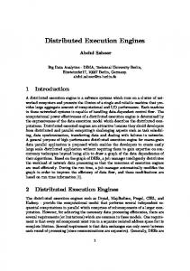
3. The Kernel of GASP 3.1. The basic kernel classes The kernel of our simulation platform offers many classes designed for an easy and safe programmation of new simulation modules. These main classes are PsSimulObject, its attributes (PsInput, PsOutput and PsCtrlParam) and the basic data types of the platform (PsType and its heirs). Now, let see what do these classes look like. The PsSimulObject class The PsSimulObject class is the main class of our simulation platform kernel. It can be viewed as the container of a calculation function Y = F(X, CP), where X is the set of inputs, Y the set of outputs and CP the set of Control Parameters

(cf figure 1). X and Y determine the data-flow from and to other objects, which can be either in the same either in another process. Each object has its own frequency and is activated periodically to compute its new state. At each simulation step, the new input values are used to compute the outputs. This requires connecting each input of the object to an output of another object. This data dependency can be static or dynamic, as we cannot know, at the beginning of a simulation, which objects will interact later. The figure 9 illustrates static data dependencies in a usual entity. To take into account dynamic data dependencies, the number of inputs of an object can change during the simulation, in contrast to the static number of outputs. PsSimulObject

PsInput

PsOutput

PsCtrlParam

PsCalculus

PsnListOfEntities

Figure 1. The OMT Diagram of PsSimulObject.

The PsType class All the basic types handled by the platform are inherited from the PsType abstract class. This ensures that those basic objects can be assigned to another instance of the same type. Then, there are some specialisation of PsType such as PsString, PsReferential, or PsNumerical. For example, PsNumerical instances authorize usual (overridden) C++ operators such as addition, substraction, division, multiplication, negation, unary and postfix increment and decrement operators ( and ++), comparison operators (, . . . ) and so on. These concrete subclasses of PsType are the ones the attributes (PsInput, PsOutput and PsCtrlParam) can handle, for example: PsInteger, PsDouble, PsString, PsRefHPR or PsList. The PsInput class A PsInput instance must be linked to a PsOutput one, in order to obtain input values for calculation. This can be done with the connect method of the PsInput class. This allows the data-flow between the two objects. When such a link is realized, the PsSimulObject only has to ask the PsInput to give him a value with the get method: the value is automatically obtained by the PsInput object from the PsOutput it is linked to. This value can then be used by the PsSimulObject object to produce a new output.

The PsOutput class We have just seen that a PsOutput instance can be linked to a PsInput one. This output is calculated by another PsSimulObject, which gives it new values using the set method. The PsCtrlParam class This class is a little bit like the PsInput one: the value of one of its instances can be obtained using its get method. The main difference is that we consider that a PsCtrlParam is local to a PsSimulObject object, so that there is no data-flow between such a PsCtrlParam instance and another object. Another difference is that the value of a PsCtrlParam can also be modified, using its set method, like a PsOutput object.


Typing the data for the computing In order to offer the greatest security for programmers, our attributes (PsInput, PsOutput and PsCtrlParam) are strongly typed: they own an instance of an heir of PsType, which can only be used to be assigned to such another object of the same type (with a get), or to which such another object of the same type can be assigned (with a set). Then, to produce computation between data of different types, for example instances of PsInteger and PsDouble, a programmer has to use basic C++ types such as int, long, float or double. We have chosen to do so because we wanted only an explicit mixing of types instead of an implicit mixing, which could have cause a lot of trouble for the modules programmers.

3.2. The implementation

heir of PsType: a PsOutput < T > will own a reference to a PsnType < T >. This PsOutput < T > will then be able to be connected to a PsInput < T > (with the connect method). The same mechanism is also used for the PsInput and PsCtrlParam classes. The main interest of our template classes is that it ensures a total type compatibility between objects linked together, for example a PsInput can only be linked with a PsOutput , and if it is not, it won’t work. It allows too the module programmer to easily use these attributes, what has already been explained. Because each simulation object has its own frequency, each attribute owns two temporal informations: the date of its last value and its production frequency. Sometimes there must be some adaptations between objects: one “client” object can ask a “server” for a value at a precise time that is not the current time in the server. It can be so because:

the server has already produced values with more recent dates; the client wants an old value (for example the value at the precedent simulation step); both the two precedent reasons.

To handle this temporal adaptation between “client” and “server” objects, we need to interpolate and extrapolate attribute values. This is possible thanks the PsnType class, as described in the next subsection. Encapsulation of the basic kernel classes Concrete PsNumerical classes are in fact instanciations of the template PsNumerical , where T stands for a basic C++ numerical type such as int and double:

; ;

typedef PsInteger PsNumerical

The PsnAttribute class and its heirs The PsInput, PsOutput and PsCtrlParam classes inherit from the PsnAttribute abstract class, which factorizes a reference to a PsSimulObject (the “owner” of the PsnAttribute), and the string representing the type of the attribute it encapsulates. We have seen that this type must be one of the kernel platform base classes, an heir of the PsType class. In order to be easily manipulated by the basic PsSimulObject instances, the PsOutput class can’t be a template one. So, it is again a virtual class, which can’t define any of the virtual methods inherited from PsnAttribute, because it only knows that the data it will encapsulate will inherit from PsType: this is in order to avoid bad manipulations between incompatible types. The most interesting method in the PsOutput class is the static one: createPsOutput which is able to create a concrete output. This concrete output will be a template heir of this PsOutput class: PsOutput < T > where T is a

typedef PsDouble PsNumerical

To encapsulate a PsType, we use the PsnType class, which is an abstract class that allows the interpolation of the encapsulated data, if the concrete heir of PsType supports it. This class uses a queue (FIFO data structure) to store old values of the data (the values at t, t - t, . . . , t n t, where t is the current time of the controller of this data, and where t is the inverse of the frequency of the controller). Thanks to this queue, it is possible to interpolate or extrapolate values not present in the queue, by an adapted approximation. The concrete classes are instances of the subclass PsnType where T stands for an heir of PsType. In fact, all the concrete instances of PsnType are obtained with a simple typedef declaration:

; ;

typedef PsnInteger PsnType typedef PsnRefHPR PsnType

3.3. Distribute the simulation

3.4. Client/Server Mechanism

The data and the streams on the network

As objects are distributed upon the network, we call reference object (PsnReference class), the reference instance as defined in the configuration file. During the simulation, the inputs of an object must be supplied with values of outputs of another object which may be located in another process. Rather than defining specifically how each reference object must send the new values of its outputs to interested reference object, an automatic mechanism has been preferred, which is based on a client/server mechanism. For each process on which the inputs of objects requires the value of the outputs of another reference object not located in the same process, an object which contains only the outputs and control parameters of the reference object is created: we call it a mirror object (PsnMirror class). Both PsnReference and PsnMirror classes inherit from the PsnCommunicating class, as shown in figure 3. The continuous communication between two agents can be managed by a two steps mechanism. Firstly, the reference object communicates to its mirror the new value of its outputs and control parameters. Secondly, the object interested by outputs or control parameters of another object can contact the embodiment of this object in its own process.

All the basic kernel classes have been designed for allowing their transport upon the network or between different processes, between different applications: all the PsType, PsnType, PsnAttribute classes inherit from a PsnFlowable abstract class, which defines two pure virtual methods extract and insert, called by the streams insertion and extraction operators: so, all its concrete subclasses will be able to be inserted into any heir of the C++ ostream class, and extracted from any heir of the C++ istream class, as they will have to implement the insert and extract methods. This allows to easily distribute the simulation.


The effective distribution A configuration file is used for each simulation to define what dynamic objects are used and on which hardware. As several processes can be used, this file describes first which processors are used, and then each process is named and located on a processor (more than one process can be located on the same processor). As the modules of an entity can be located in separate processes, the location of each module is specified in the configuration file. In the example of the figure 2, driver1 is an instance of the class CAR DRIVER and also a part of the entity named car1. driver1 is located on the process P2 which is himself located on the machine goudurix. Each instance can be created with specific initial data, given in the configuration file. For example, at the creation of geomecha1, a geometric model is associated (an OpenInventor file) and an initial location is given (X, Y, Z and orientation values). //GASP configuration file processes: //machine_name process_name indefix P1 goudurix P2 onyx P3 simulation_objects: //FatherName ClassName Name Process Frequency root ENTITY car1 root VISUALIZATION visu P3 50 car1 HUMAN_VISION vision1 P1 10 car1 CAR_DRIVER driver1 P2 10 car1 CAR_CONTROLLER llc1 P2 100 car1 CAR_GEO_MECHA geomecha1 P1 100 //Initial values parameters: geomecha1 data/car.iv 10.0 0.0 20.0 90.0 visu data/scene.iv driver1 1

Figure 2. An example of configuration file.

PsnMessage

PsnCommunicating

PsnMirror

PsSimulObject

PsnReference

Figure 3. OMT Diagram of the class PsnCommunicating.

Local Controller

Local Controller IP Channel Receive

Send

Subscribe

X.reference

Unsubscribe X.mirror

Process 1

Process 2

Figure 4. Communication between reference and mirror objects.

As each reference object runs at its own internal frequency, the data-flow communication channel must include all the mechanisms to adapt to the local frequency of the producer and of consumers (over-sampling, sub-sampling, interpolation and extrapolation). With the intention of minimizing communications between processes, the frequency

of the communication (fC ) between a reference object and each of its mirrors is computed especially for each mirror, and it depends on two kinds of information: the frequency of the reference object (fR ) and the maximum frequency of the reference objects located on the same process than the mirror (fM ). If fR < fM then fC = fR else fC is the lowest sub-multiple of fR which is higher than fM (cf figure5). Fm >= Fr P1 Freq = 100HZ

P2 Freq = 150HZ A.Ref Freq = 50HZ

D.Ref Freq = 100HZ

C.Mir IP Channel Fc = 20HZ

C.Ref Freq = 20HZ Fm < Fr P1 Freq = 1100HZ

P2 Freq = 150HZ A.Ref C.Mir Freq = 50HZ

D.Ref Freq = 50HZ IP Channel Fc = 55HZ

C.Ref Freq = 220HZ


B.Ref Freq = 30HZ

Fm = 50HZ

B.Ref Freq = 30HZ

Fm = 50HZ

Figure 5. Communication frequencies between a reference object C and its mirrors. Figure 6 illustrates the simulation sub-trees existing during a simulation on each process, on the basis of the configuration file described in figure 2. P1

vision1

P2

root

root

car

car

driver1

llc1

vision1

geomecha1

llc1

driver1

geomecha1

P3 Reference Object

root

work, so it limits our cooperative capabilities to workstations and parallel machines over the same local area network.

3.5. Local Controllers Each process owns its own local controller to manage the synchronization and the execution of all its reference objects. The frequency of the Local Controller is the lowest common multiple of its reference objects frequencies. This controller follows a regular cycle composed of six different phases: 1. receive inter-processes messages; 2. ask each addressee object to receive its messages; 3. ask each activated reference object to compute a simulation step; 4. ask the same reference objects to emit a message containing the new values of their outputs; 5. ask each object to emit its event based messages; 6. emit inter-process messages. The IPChannel class is used to manage inter-process communication. It regroups all messages that must be exchanged between two processes (messages between reference and mirror objects, and sporadic events). Insertion and extraction operators for the PsnMessage class are available, allowing the insertion of any PsFlowable object into a PsnMessage, and the extraction of any PsFlowable object from a PsnMessage. This is possible because the PsnMessage class owns an input stream and an output stream. The global synchronization between local controllers is assumed by a global controller which performs a global synchronization every K seconds (K is an integer 1).

3.6. Interprocess Communication

Mirror Object car

visu

geomecha1

Figure 6. Simulation sub-trees on different processes. This approach is quite different from the one chosen by NPSNET [13] which enables cooperative work all over the internet by sending “ghosts” (mirror representations of the references), with simplified behaviour regularly synchronized, to interested applications (dead-reckoning and synchronization multicasting). Our data-flow approach is more efficient for real-time interaction as it allows a better synchronization. Nevertheless, it needs a larger bandwith net-

The distribution of the entities in different processes and their communication is realized using PVM (Parallel Virtual Machine) [12]. PVM is a software package which permits to develop parallel programs executable on networked Unix computers. It allows a heterogeneous collection of workstations and supercomputers to function as a single highperformance parallel machine. It is portable ans runs on a wide variety of modern platforms. In PVM, we describe an application as a collection of cooperating tasks. Tasks access PVM resources through a library of standard interface routines. These routines allow the initiation and termination of tasks across the network as well as communication and synchronization between tasks. The PVM message-passing primitives involve strongly typed constructs for buffering and transmission. Communication constructs include those for sending and receiving data structures. In our case, the global controller spawns a process with a local controller

on the different workstations declared in the configuration file.

4. Module Programming 4.1 Introduction In this section, we will illustrate what should be performed by a programmer to describe his own module in GASP. Each module should be described by two classes: the first one, which should be derived from the PsSimulObject Class, defines the interface of the module with the external world, while the second class, which should be derived from the PsCalculus Class, specifies how to perform a simulation step. The figure 7 shows attributes and methods of the two classes to be specialized by a programmer to define a specific module.


PsSimulObject arrayOfInputs : PsArrayRefObject arrayOfOutputs : PsArrayRefObject arrayOfCtrlParams : PsArrayRefObject communicating: * PsCommunicating controller: * PsLocalController initArrayOfInputs() {virtual} initArrayOfOutputs() {virtual} initArrayOfCtrlParams() {virtual} createCalculus(): * PsCalculus {virtual} initListOfSubObjects(PsListClass *list) {virtual} associateCode(int i) {virtual} createObjectCode(PsClass class): * PsSimulObject addInput(PsSymbName name, PsTypeAtt type) addOutput(PsSymbName name, PsTypeAtt type) addCtrlParam(PsSymbName name, PsTypeAtt type) refOutput(PsSymbName nameAtt): * PsOutput refInput(PsSymbName nameAtt): * PsInput refCtrlParam(PsSymbName nameAtt): * PsCtrlParam

PsCalculus simulObject: * PsSimulObject init() {virtual} calculate(){virtual} end(){virtual}

Figure 7. Attributes and methods of PsSimulObject and PsCalculus classes.

4.2 Defining one’s own specialization of PsSimulObject The class PsSimulObject contains five virtual methods that must be defined for each specialization. Three of them (initArrayOfInputs(), initArrayOfOutputs() and initArrayOfCtrlParams()) are used to declare the initial

sets of inputs, outputs and control parameters, by using the three methods addInput, addOutput and addCtrlParam. The number of inputs can be dynamically modified during the simulation unlike the one of outputs, so it is necessary to define all outputs in the method initArrayOfOutputs(). Each attribute must be specified by a symbolic name, a type of data and an interpolation level (only for inputs): void myObject::initArrayOfInputs () { addInput(new PsInput ("distance", MAX_INTERPOL)); ... } void myObject::initArrayOfOutputs () { addOutput(new PsOutput ("brake_indicator")); ... }

The two other methods are used to declare sub-objects (initListOfSubObjects()) and to create and make a link to a PsCalculus object (createCalculus()). PsCalculus *myObject::createCalculus () { return new myObjectCalculus (); }

4.3 Defining one’s own calculation function Due to the reference/mirror mechanism, the PsSimulObject class delegates to the PsCalculus class the calculation of the simulation steps, which avoids the duplication of the calculation function on the mirror objects. The PsCalculus class is used to define the calculation function by using three methods init(), calculate() and end(), which correspond to the initialization, the simulation step and the termination of the simulation algorithm. To connect an input of a module to an output of another module, we should be sure that the outputs of the second one has already been created. This is why we have to perform the first connections in the init() method of the PsCalculus object. As inputs can be created at anytime during the simulation, their connection can also be performed or modified whenever we want during the simulation. Class myObjectCalculus: public PsCalculus { public: void init (); private: PsInput *v; }; void myObjectCalculus::init () { v->connect("another_object", "an_output", MAX_INTERPOL); ... }

In this connection, the symbolic name of the other object and of its output are given, but other kinds of connection are available, especially by using a reference instead of a symbolic name either for the object or for the output 1 . The 1 This

is useful when we use the simulation tree to search an object

level of interpolation indicates if data will be estimated or if the preceding data will be given at intermediate times. Four levels of interpolation are available: none, linear, quadratic and cubic. This allows to estimate the value of the output (only for PsFloat and PsDouble types of data) at other dates than the produced one 2 .

4.4 Creating sub-objects Each module can itself create some sub-objects, which will become its sons in the simulation tree. Two virtual methods of the PsSimulObject class should be redefined by the programmer: initListOfSubObjects(PsListClass *list) fvirtualg associateCode(int i) fvirtualg


Let us present an example of how these methods are used: Class myObject: public PsSimulObject { public: void initListOfSubObjects(PsListClass *); PsSimulObject *associateCode (int); Private: Enum sons {SUBOBJ1, SUBOBJ2} }; void myObject::initListOfSubObjects (PsListClass *list) { list->addClass(SUBOBJ1, "Subobj1"); list->addClass(SUBOBJ2, "Subobj2"); } PsSimulObject *myObject::associateCode (int i) { switch (i) { case SUBOBJ1 : return new subObj1 (); case SUBOBJ2 : return new subObj2 (); // ............ } return NULL; }

At the beginning of a simulation, sons of the root of the simulation tree should be created. To associate objects to the root, the programmer has to use the same two methods in the PsTheListOfEntities class.

Figure 8. One shot from a simulation.

DIATS. DIATS is a research project sponsored by the European Community. It aims at defining and studying some ATT (Advanced Transport Telematics) scenarios on interurban motorways. As a matter of fact the problems of congestion arising from an increasing number of vehicles on the roads have focused Government Policies towards a more efficient management of the existing road network. We are currently coding different ATT systems including AID (Automatic Incident Detection), variable speed limits, ramp metering, AICC (Autonomous Intelligent Cruise Control), inside GASP to be able to evaluate the impact of each of them on congestion problems. Multimodal Traffic Simulation in Urban Cities. An implementation of a virtual driver has been performed and tested (cf figure 8). We are currently working on an interactive behaviour modelling system able to specify and generate different kinds of virtual drivers for GASP (car driver, truck driver, bicycle driver, pedestrians. . . ).

5. Example of Behavioural Simulation Entity

5.1 A Driving Simulation Example GASP has been used for several projects in the field of driving simulation: Praxitele Project. Simulation of a fleet of small electric vehicles, which can be automatically driven on specific journeys: platooning, parking [2]. 2 This

is useful to manage communication delay between processes

Sensor

Driver

Low Level

Geo-Mecha

Motion Control

Model

Data Dependency

Figure 9. Structural view of a usual entity.

x, y, theta

Visual

x_camera, y_camera, theta_camera Lane pLWarn pRWarn

Pool

1 listDynObj listSigType listSigNum listSigDist

State

Entity

2

action xtarget ytarget distance speed headway Objname

Grid ex, etheta ey, state

Sensor

3

state

Pilot

4

motor torque brake

LLC

5

RedLight WarnLight (x4) x, y, z gamma eps phi (x4) chassis body wheel (x4) GeoMecha

7

6 a, b, theta

state state

a, b, theta, beta

pa, pb, ptheta

LWarn, RWarn

state a, b, theta Link to another vehicle Several instances

1 time step delay Data flow

Unique instance

1

Link through pointer

Execution order


Figure 10. Architecture of the automated car driver simulation loop. Each entity is composed of several modules. For example, a car is composed of five different kinds of Modules, as shown in figure 9. In the field of real-time animation or simulation, it is impossible to completely simulate human vision and the building of a mental model of the environment. Therefore, the automatic driver gets a local view of its environment through a sensor which is in fact a filter of the whole environment database. Two different types of objects are taken into account in the sensor: static objects (buildings, road signals, traffic lights) and dynamic objects (cars, trucks, bicycles). Objects that would be hidden by closer objects are eliminated thanks to a Z-buffer algorithm. The goal of the decisional model (driver) is to produce a target point and an output action with parameters for the low-level controller. These actions include a normal free driving mode at a desired speed, a following mode and different breaking modes. The goal of the low-level controller is to produce a guidance torque, an engine torque and a brake pedal pressure as inputs for the mechanical model. The mechanical aspect of the car is modelled with DREAM [8], our rigid and deformable bodies modeling systems. By means of Lagrange’s equations, DREAM computes exact motion equations in a symbolic form for analysis and then generates numerical C++ simulation code for GASP. The module which represents the behavioural model is presented in more details to illustrate the capabilities and the usability of GASP. This module is connected to different other modules as shown in the figure 10. The behavioural model (Pilot module) receives different lists from the sensor indicating static and moving visible objects (cf figure 11). From the geo-mechanical module (generative model), it re-

Name a b theta ListDynObj ListSigType ListSigNum ListSigDist pa pb ptheta lane pLWarn pRWarn

Type PsDOUBLE PsDOUBLE PsDOUBLE PsLIST PsSTRING PsLIST PsINTEGER PsLIST PsINTEGER PsLIST PsFLOAT PsDOUBLE PsDOUBLE PsDOUBLE PsINTEGER PsINTEGER PsINTEGER

< < <
> > >

Meaning X coordinate of the car Y coordinate of the car orientation of the car list of moving object names) list of vertical road-signs types list of vertical road-signs number list of distances to vertical road-signs X coordinate of another vehicle Y coordinate of another vehicle orientation of another vehicle lane of another vehicle left turning light of another vehicle right turning light of another vehicle

Figure 11. Inputs of the Pilot object.

ceives also the current location of its own vehicle, but also of other visible vehicles. The visual class is a generic Performer viewer which is able to animate the geometric model of each dynamic object. That is the reason why we have added some specific types of data into GASP, like PsReferential heirs with different degrees of freedom in rotation and translation or PsSwitch. The main outputs of the driver (cf figure 12) describe actions which should be performed by the low level motion controller, like for example: “Follow the preceding vehicle with a desired headway of 0.8s and switch on the left turning light”. The control parameters (cf figure 13) are used to characterise each embodiment of the class, but they can be modified during the simulation like the status parameter which switchs from idle to semi-active, then to active and finally to terminated. Another status reachable at anytime is accident, because an accident can occur due to the responsibility of

Name action distance speed headway Objname xtarget ytarget LWarn RWarn x camera y camera theta camera lane

Type PsINTEGER PsDOUBLE PsDOUBLE PsDOUBLE PsSTRING PsDOUBLE PsDOUBLE PsINTEGER PsINTEGER PsDOUBLE PsDOUBLE PsDOUBLE PsINTEGER

Description action to perform stopping distance desired speed desired headway name of the vehicle to follow X coordinate of the target Y coordinate of the target left turning light right turning light X coordinate of the visual sensor Y coordinate of the visual sensor orientation of the visual sensor lane number

Figure 12. Outputs of the Pilot object. Name status desired speed desired headway

Type PsINTEGER PsDOUBLE PsDOUBLE

Description status of the vehicle desired speed of the vehicle desired headway of the vehicle


Figure 13. Control Parameters of the Pilot object.

another vehicle. The heir of the PsCalculus object implements the decisional model of the car driver. It is automatically generated by a tool which transforms a model described as a Hierarchical Parallel Transition System (HPTS) into its C++ implementation inside GASP [9]. This model is both cognitive and reactive including synchronous data-flow and asynchronous event based communications.

6. Conclusion. In this paper, we have presented GASP: a General Animation and Simulation Platform which enables a modular specification of animation and which takes the execution and synchronization tasks from the activity of a module programmer. This platform enables:

modular specification of simulations; integration of descriptive, generative and behavioural models; massive distribution of objects upon heterogeneous workstations; data-flow communication with frequency adaptation mechanisms; synchronization of the distributed objects;

without any trouble from the module programmer’s point of view. For the DIATS project we have performed some simulations including 2800 of such vehicles evolving on a 6 Km long highway road.

References [1] O. Ahmad, J. Cremer, S. Hansen, J. Kearney, and P. Willemsen. Hierarchical, concurrent state machines for behavior modeling and scenario control. In Conference on AI, Planning, and Simulation in High Autonomy Systems, Gainesville, Florida, USA, 1994. [2] B. Arnaldi, R. Cozot, S. Donikian, and M. Parent. Simulation models for the french praxitele project. In Transportation Research Board Annual Meeting, Washington DC, USA, Jan. 1996. [3] N. I. Badler, C. B. Phillips, and B. L. Webber. Simulating Humans : Computer Graphics Animation and Control. Oxford University Press, 1993. [4] N. I. Badler, B. L. Webber, J. Kalita, and J. Esakov, editors. Making them move: mechanics, control, and animation of articulated figures. Morgan Kaufmann, 1991. [5] B. Blumberg and T. Galyean. Multi-level direction of autonomous creatures for real-time virtual environments. In Siggraph, pages 47–54, Los Angeles, California, U.S.A., Aug. 1995. ACM. [6] W. Bricken and G. Coco. The VEOS project. Presence, 3(2):111–129, 1994. [7] A. Chauffaut and S. Donikian. Gasp: a general animation and simulation platform. In ISMCR’97, XIV IMEKO World Congress, Tampere, Finland, June 1997. [8] R. Cozot. From multibody systems modelling to distributed real-time simulation. In ACM, editor, American Simulation Symposium, New Orleans, USA, 1996. [9] S. Donikian. Multilevel modeling of virtual urban environments for behavioural animation. In Computer Animation’97, Geneva, Switzerland, June 1997. IEEE Computer Society Press. [10] S. Donikian and R. Cozot. General animation and simulation platform. In D. Terzopoulos and D. Thalmann, editors, Computer Animation and Simulation’95, pages 197– 209. Springer-Verlag, 1995. [11] S. Donikian and E. Rutten. Reactivity, concurrency, dataflow and hierarchical preemption for behavioural animation. In E. B. R.C. Veltkamp, editor, Programming Paradigms in Graphics’95, Eurographics Collection. Springer-Verlag, 1995. [12] A. Geist, A. Beguelin, J. Dongarra, W. Jiang, R. Manchek, and V. Sunderam. PVM: Parallel Virtual Machine. The MIT Press, 1994. [13] M. Macedonia, D. Brutzman, M. Zyda, D. Pratt, P. Barham, J. Falby, and J. Locke. NPSNET: a multi-player 3d virtual environment over the internet. In Symposium on Interactive 3D Graphics, Monterey, California, Apr. 1995. ACM.