Coding and Iterative Decoding of Concatenated

Coding and Iterative Decoding of Concatenated Multi-level Codes for the Rayleigh Fading channel

OMAR AL-ASKARY

Doctoral Thesis in Radio Communication Systems Stockholm, Sweden 2006

Coding and Iterative Decoding of Concatenated Multi-level Codes for the Rayleigh Fading channel

OMAR AL-ASKARY

Doctoral Thesis in Radio Communication Systems Stockholm, Sweden 2006

TRITA–ICT–COS–0603 ISSN 1653–6347 ISRN KTH/RST/R--06/03--SE

KTH Communication Systems SE-100 44 Stockholm SWEDEN

Akademisk avhandling som med tillst˚ and av Kungl Tekniska högskolan framl¨ agges till offentlig granskning för avläggande av teknologie doktorsexamen den 12 juni 2006, klockan 13.00 i sal C1, Electrum, Isafjordsgatan 22, Kista. c Omar Al-Askary, June 2006

Tryck: Universitetsservice US-AB

Abstract In this thesis we present the concept of concatenated multilevel codes. These codes are a combination of generalized concatenated codes with multilevel coding. The structure of these codes is simple and relies on the concatenation of two or more codes of shorter length. These codes can be designed to have large diversity which makes them attractive for use in fading channels. We also present an iterative decoding algorithm taylored to fit the properties of the proposed codes. The iterative decoding algorithm we present has a complexity comparable to the complexity of GMD decoding of the same codes. However, The gain obtained by using the iterative decoder as compared to GMD decdoing of these codes is quite high for Rayleigh fading channels at bit error rates of interest. Some bounds on the performance of these codes are given in this thesis. Some of the bounds are information theoretic bounds which can be used regardless of the code under study. Other bounds are on the error probability of concatenated multilevel codes. Finally we give examples on the implementation of these codes in adaptive coding of OFDM channels and MIMO channels.

iii

Acknowledgements The work with my thesis was long and hard. I have learned two important things when I was working with the thesis. The first is that the more you learn the more you understand that there is much more to learn. The second thing is that there are people who are willing to teach you and help you in your work. In my case, I am indebted to my colleagues at Radio Systems group who helped make my work succeed. Special thanks to Professor Slimane Ben Slimane, my adviser, for his guidance. Many thanks to Professor Jens Zander for his support. I am endlessly grateful to Lise-Lotte Wahlberg for the extensive help in clearing the practical and administrative details. Lise-Lotte’s sisterly caring for all the employees in the group makes her an invaluable asset. Thanks also to Irina Radulescu for all the help with the practicalities of printing the thesis. Many thanks go to Niklas Olsson for his help regarding the computer system and for always being patient regardless how stupid a problem is. Thanks also to Klas Johansson and Bogdan Timus for proofreading the thesis. Thanks also to Mats Blomgren for helping me check the format and other possible deficiencies in the final document. I shouldn’t forget all my other colleagues in Radio Systems group for their feedback. Special thanks to Professor Joachim Hagenauer for his valuable comments and feedback.

v

To Wafaa, Muhammad-Ali and Maryam. sorry for all the inconvenience1

1 Douglas

Adams. Hitchhiker’s Guide to the Galaxy. God’s last message to the Universe.

vii

Contents 1 Introduction

1

1.1

Background . . . . . . . . . . . . . . . . . . . . . . . . . . . . . . . .

1

1.2

Communications over the wireless channel . . . . . . . . . . . . . . .

2

1.3

Channel coding and concatenated codes . . . . . . . . . . . . . . . .

3

1.4

Related work . . . . . . . . . . . . . . . . . . . . . . . . . . . . . . .

5

1.5

Contribution and outline of the thesis . . . . . . . . . . . . . . . . .

6

2 Preliminaries

I

11

2.1

System Model . . . . . . . . . . . . . . . . . . . . . . . . . . . . . . . 11

2.2

Channel capacity . . . . . . . . . . . . . . . . . . . . . . . . . . . . . 18

2.3

Evaluating the performance of codes . . . . . . . . . . . . . . . . . . 19

Information theoretic aspects

3 Capacity of the Rayleigh fading channel with error in CSI

23 25

3.1

Introduction . . . . . . . . . . . . . . . . . . . . . . . . . . . . . . . . 25

3.2

System model . . . . . . . . . . . . . . . . . . . . . . . . . . . . . . . 26

3.3

Capacity calculation . . . . . . . . . . . . . . . . . . . . . . . . . . . 28

3.4

Optimizing the constellations by genetic algorithms . . . . . . . . . . 32 ix

x

Contents

3.5

Numerical results and discussion . . . . . . . . . . . . . . . . . . . . 34

4 Bounds on the capacity of the Rayleigh fading channel with error in CSI 43 4.1

The Rayleigh fading channel with error in CSI and an optimal receiver 44

4.2

The scaled output channel with error in CSI . . . . . . . . . . . . . . 49

4.3

Examples and Discussion . . . . . . . . . . . . . . . . . . . . . . . . 56

5 Capacity of the fading channel with silence and the ignoring receiver 59

II

5.1

Constellation capacities for the channel with silence and for the ignoring receiver with an optimal decoder . . . . . . . . . . . . . . . . 62

5.2

Constellation capacities for the channel with silence, ignoring receiver and a scaled output decoder . . . . . . . . . . . . . . . . . . . 65

5.3

Discussion . . . . . . . . . . . . . . . . . . . . . . . . . . . . . . . . . 69

Concatenated multilevel codes: General properties

6 Definition of Concatenated Multilevel Codes

71 73

6.1

Product codes and concatenated codes . . . . . . . . . . . . . . . . . 74

6.2

Proposed concatenated multilevel codes . . . . . . . . . . . . . . . . 77

6.3

Properties of concatenated multilevel codes . . . . . . . . . . . . . . 77

6.4

Methods for decoding concatenated codes . . . . . . . . . . . . . . . 81

7 Iterative decoding of concatenated multilevel codes

89

7.1

A maximum likelihood decoder for product codes . . . . . . . . . . . 90

7.2

Iterative low complexity decoding . . . . . . . . . . . . . . . . . . . . 91

7.3

Error correction capability of the suboptimal algorithm . . . . . . . 96

7.4

Decoding the constituent codes . . . . . . . . . . . . . . . . . . . . . 104

7.5

Increasing the speed of convergence . . . . . . . . . . . . . . . . . . . 106

Contents

xi

7.6

Complexity of decoding . . . . . . . . . . . . . . . . . . . . . . . . . 111

7.7

Simple measure of the decoding complexity . . . . . . . . . . . . . . 117

8 Performance of the iterative decoding algorithm

119

8.1

Product codes on BSC . . . . . . . . . . . . . . . . . . . . . . . . . . 119

8.2

Product codes on AWGN channel . . . . . . . . . . . . . . . . . . . . 122

8.3

A concatenated multilevel code on the AWGN channel . . . . . . . . 126

8.4

Concluding remarks . . . . . . . . . . . . . . . . . . . . . . . . . . . 126

9 Bounds on the block error probability

129

9.1

Upper bounds on block error probability for product codes

. . . . . 129

9.2

Application to concatenated multilevel codes . . . . . . . . . . . . . 149

9.3

Lower bounds on the error probability . . . . . . . . . . . . . . . . . 157

9.4

An approximate bound on the block error probability for the Rayleigh fading channel . . . . . . . . . . . . . . . . . . . . . . . . . . . . . . 161

9.5

Summary . . . . . . . . . . . . . . . . . . . . . . . . . . . . . . . . . 161

III Concatenated multilevel codes: Design for Rayleigh fading channels 165 10 Construction and decoding

167

10.1 Choosing the rates of the constituent codes. . . . . . . . . . . . . . . 167 10.2 Multilevel code construction . . . . . . . . . . . . . . . . . . . . . . . 170 10.3 Choice of the decoder . . . . . . . . . . . . . . . . . . . . . . . . . . 173 10.4 Decoding on fading channels . . . . . . . . . . . . . . . . . . . . . . . 174 10.5 Effect of imperfect channel state information . . . . . . . . . . . . . 175 11 Performance

177

11.1 A detailed examination of a code example . . . . . . . . . . . . . . . 178

xii

Contents

11.2 Different examples of performance of concatenated multilevel codes . 184 11.3 Effect of CSI error on performance . . . . . . . . . . . . . . . . . . . 187 11.4 Measured decoding complexity . . . . . . . . . . . . . . . . . . . . . 189 11.5 summary . . . . . . . . . . . . . . . . . . . . . . . . . . . . . . . . . 193 12 Adaptive Coding for OFDM Based Systems using Generalized Concatenated Codes 195 12.1 Introduction . . . . . . . . . . . . . . . . . . . . . . . . . . . . . . . . 195 12.2 System . . . . . . . . . . . . . . . . . . . . . . . . . . . . . . . . . . . 196 12.3 Modulation and Coding . . . . . . . . . . . . . . . . . . . . . . . . . 197 12.4 Application to H/2 . . . . . . . . . . . . . . . . . . . . . . . . . . . . 201 12.5 Simulation Model . . . . . . . . . . . . . . . . . . . . . . . . . . . . . 202 12.6 Results . . . . . . . . . . . . . . . . . . . . . . . . . . . . . . . . . . . 204 12.7 Conclusions . . . . . . . . . . . . . . . . . . . . . . . . . . . . . . . . 205 13 Adaptive Generalized Concatenated Codes for MIMO Communication 207 13.1 Introduction . . . . . . . . . . . . . . . . . . . . . . . . . . . . . . . . 207 13.2 System Model . . . . . . . . . . . . . . . . . . . . . . . . . . . . . . . 209 13.3 Rate Adaptive Code Construction . . . . . . . . . . . . . . . . . . . 219 13.4 Simulation Results . . . . . . . . . . . . . . . . . . . . . . . . . . . . 222 13.5 Conclusion

. . . . . . . . . . . . . . . . . . . . . . . . . . . . . . . . 223

14 Conclusions and future work

231

14.1 Summary and conclusions . . . . . . . . . . . . . . . . . . . . . . . . 231 14.2 Future work . . . . . . . . . . . . . . . . . . . . . . . . . . . . . . . . 233 A Proof of Lemma 9.9

235

A.1 The concept of constructing rectangles . . . . . . . . . . . . . . . . . 235

Contents

xiii

A.2 The suboptimal decoder . . . . . . . . . . . . . . . . . . . . . . . . . 244 B The Complex Cauchy Distribution

249

C Sorting Algorithms λ and µ

255

References

259

List of Figures 2.1

Model of the system used in the thesis . . . . . . . . . . . . . . . . . 12

3.1

Genetic algorithm . . . . . . . . . . . . . . . . . . . . . . . . . . . . 33

3.2

The constellation capacity of QPSK for the optimum decoder, (3.12) and the scaled output channel (3.21). . . . . . . . . . . . . . . . . . . 34

3.3

The constellation capacity of 8PSK for the optimum decoder, (3.12) and the scaled output channel (3.21). . . . . . . . . . . . . . . . . . . 35

3.4

The constellation capacity of 16QAM for the optimum decoder, (3.12) and the scaled output channel (3.21). . . . . . . . . . . . . . . 36

3.5

The constellation capacity of 32QAM for the optimum decoder, (3.12) and the scaled output channel (3.21). . . . . . . . . . . . . . . 36

3.6

The constellation capacity of QPSK for the optimum decoder, (3.12) compared to Algorithm 3.1. . . . . . . . . . . . . . . . . . . . . . . . 37

3.7

The constellation capacity of 8PSK for the optimum decoder, (3.12) compared to Algorithm 3.1. . . . . . . . . . . . . . . . . . . . . . . . 37

3.8

The constellation capacity of 16QAM for the optimum decoder, (3.12) compared to Algorithm 3.1. . . . . . . . . . . . . . . . . . . . 38

3.9

The constellation capacity of 32QAM for the optimum decoder, (3.12) compared to Algorithm 3.1. . . . . . . . . . . . . . . . . . . . 38

2 3.10 Signal constellation obtained by Algorithm 3.1. SNR = 20 dB, σw = 0 39 2 = 3.11 Signal constellation obtained by Algorithm 3.1. SNR = 0 dB, σw 0.25 . . . . . . . . . . . . . . . . . . . . . . . . . . . . . . . . . . . . 40

xv

xvi

List of Figures

2 3.12 Signal constellation obtained by Algorithm 3.1. SNR = 0 dB, σw = 0.75 . . . . . . . . . . . . . . . . . . . . . . . . . . . . . . . . . . . . 40 2 = 3.13 Signal constellation obtained by Algorithm 3.1. SNR = 20 dB, σw 0.25 . . . . . . . . . . . . . . . . . . . . . . . . . . . . . . . . . . . . 41 2 3.14 Signal constellation obtained by Algorithm 3.1. SNR = 20 dB, σw = 0.75 . . . . . . . . . . . . . . . . . . . . . . . . . . . . . . . . . . . . 41

3.15 The maximum possible constellation capacity of 32 signal constellation compared with mutual information of a Gaussian codebook. . . 42 4.1

The upper and lower bounds on constellation capacity for the optimal receiver case. . . . . . . . . . . . . . . . . . . . . . . . . . . . . . 56

4.2

The upper and lower bounds on constellation capacity for the optimal receiver case. . . . . . . . . . . . . . . . . . . . . . . . . . . . . . 57

5.1

Three different channel models to use the channel estimate. . . . . . 61

5.2

constellation capacity for the channel with silence and optimal decoder for QPSK modulation . . . . . . . . . . . . . . . . . . . . . . . 63

5.3

The threshold for silence vs. SNR. . . . . . . . . . . . . . . . . . . . 64

5.4

constellation capacity for the channel with ignoring receiver with QPSK modulation and optimal decoder . . . . . . . . . . . . . . . . 65

5.5

constellation capacity for the channel with silence and optimal decoder for QPSK modulation . . . . . . . . . . . . . . . . . . . . . . . 67

5.6

The threshold for silence vs. SNR for scaled output receiver . . . . . 68

5.7

constellation capacity for the channel with ignoring receiver with QPSK modulation and optimal decoder . . . . . . . . . . . . . . . . 68

6.1

Construction of product codes . . . . . . . . . . . . . . . . . . . . . . 74

6.2

Constructing a three level multilevel code from a GCC. . . . . . . . 78

6.3

Trellis of the [7, 4, 3] Hamming code. . . . . . . . . . . . . . . . . . . 83

7.1

List decoding of the codes A and B. . . . . . . . . . . . . . . . . . . 91

7.2

Decoding stages of the iterative decoder . . . . . . . . . . . . . . . . 92

List of Figures

xvii

7.3

The iterative, suboptimal algorithm for decoding product codes. . . 94

7.4

Correction of burst errors. . . . . . . . . . . . . . . . . . . . . . . . . 97

7.5

Proof of Theorem 7.3. . . . . . . . . . . . . . . . . . . . . . . . . . . 100

7.6


7.7


7.8

Worst case of an error pattern of weight
tol do i ← i + 1; L ← Y + Li−1 ; Generate the children of the survivor constellation. The average power of the children are kept the same as the parent; Li ← arg maxL′ ∈L C(L′ ); e ← |C(Li ) − C(Li−1 )|; end end Figure 3.1: Genetic algorithm

and thus the capacity is the normal distribution. When the CSI is totally unknown at the receiver, Shamai et al [60] proved that optimum distribution is a discrete distribution that is different for different value of the signal to noise ratio. The question what is the optimum probability distribution of the signal for the channel with error in CSI and for different values of signal to noise ratios is difficult to answer in general. We try, on the other hand, to answer a simpler question. We try to maximize the mutual information given by (3.8), between the input and the output of the channel by considering all possible signal constellations of a certain number of signals. The PDF of the received signal is changed accordingly by using (3.17) for the optimal decoder channel and (3.22) for the scaled output receiver channel. To explain in more detail, assume that we consider the family of all signal constellations of cardinality q where all signal points have equal probability. We try to find the maximum mutual information that can be obtained of this family of constellations. We use a genetic algorithm [65], [66] to find a constellation that maximizes the mutual information. It is evident that the result is actually a lower bound and not the actual maximum even though it is a good lower bound. In Figure 3.1 we show the genetic algorithm used to find the constellation that has a constellation capacity approaching the maximum that can be obtained from this family of constellations.

34

Chapter 3. Capacity of the Rayleigh fading channel with error in CSI.

In the results given in this work, we added one more limitation to the structure of the constellations that maximize the mutual information. The limitation is that the constellation should be made of pairs of points such that each pair is symmetrical around the origin. There was no noticeable difference between the results for the case when this limitation was removed and the results when it was added. This symmetry makes the constellations easier to understand and to have an idea about their meaning.

3.5

Numerical results and discussion

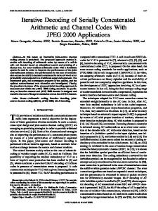
As mentioned above, we investigate the constellation capacity for the some of the popular modulation methods such as PSK and QAM. We, therefore, compare the constellation capacities of these modulation methods with the maximum possible mutual information that can be achieved by a constellation of the same cardinality obtained using the genetic algorithm above. We begin by comparing the constellation capacities for the optimal decoder and the scaled output channel for different types of modulation and estimation error. In Figure 3.2 we see the constellation capacity for QPSK modulation for the two channel types. We notice that for both channels there exists a certain upper value 2 σ =0 w

Optimal Scaled

1.8 1.6

C bits/transmission

1.4

σ =0.25 w

σ =0.5

1.2

w

1 0.8 0.6 σ =0.75

0.4

w

0.2 0

0

2

4

6

8

10 SNR dB

12

14

16

18

20

Figure 3.2: The constellation capacity of QPSK for the optimum decoder, (3.12) and the scaled output channel (3.21). that the capacity approaches. This upper value decreases when the error in estimation is increased. For the case when there is no estimation error, the capacity

3.5. Numerical results and discussion.

35

for both channels approach the maximum bit rate that can be obtained by using QPSK modulation, i.e., 2 bits/transmission. However, when the estimation error increases, the constellation capacity for the scaled output channel is affected much more severely than for the optimal receiver. The same observations are made for the other modulation types such as 8PSK in Figure 3.3, 16QAM in Figure 3.4 and 32QAM in Figure 3.5. We now compare the constellation capacities for cer3 Optimal Scaled

2.5

σ =0

C, bits/transmission

w

σ =0.25

2

w

1.5 σw=0.5 1

0.5

σ =0.75 w

0

0

2

4

6

8

10 SNR, dB

12

14

16

18

20

Figure 3.3: The constellation capacity of 8PSK for the optimum decoder, (3.12) and the scaled output channel (3.21). tain modulation types with the maximum possible constellation capacity that can be obtained for any constellation that of the same cardinality as the modulation method under study. We first investigate the case for the optimal decoder. In Figure 3.6 we see a comparison between the constellation capacity of the QPSK modulation and the maximum possible constellation capacity of a four signal point constellation obtained using Algorithm 3.1. In Figure 3.7 we see the comparison between the constellation capacity for 8PSK modulation and the maximum possible constellation capacity of an 8 signal constellation. In Figures 3.8 and 3.9 the same comparison is made for 16QAM modulation and the 32QAM modulation respectively. We notice that the upper limit on the constellation capacity is much greater for the maximum possible constellation capacity acquired via the genetic algorithm in Algorithm 3.1 than that for the usual modulation methods investigated. The maximum constellation capacity seems to approach the bandwidth efficiency of the constellation for no error estimation case. I.e., the maximum achievable constellation capacity seems to approach log q, where q is the number of signals in the signal constellation. It is quite clear from the figures above, that the QAM modulation is less prone to the error in the CSI. The explanation to that can be made

36


4

3.5

Optimal Scaled σw=0


3

σ =0.25

2.5

w

2 σ =0.5 w

1.5

1

σ =0.75

0.5

0

w

0

2

4

6

8

10 SNR, dB

12

14

16

18

20

Figure 3.4: The constellation capacity of 16QAM for the optimum decoder, (3.12) and the scaled output channel (3.21).

4.5 Optimal Scaled 4

3.5


3

σw=0 σw=0.25

2.5

2 σw=0.5 1.5

1 σw=0.75

0.5

0

0

2

4

6

8

10 SNR, dB

12

14

16

18

20

Figure 3.5: The constellation capacity of 32QAM for the optimum decoder, (3.12) and the scaled output channel (3.21).


37

2 σw=0.75

Genetic Alg QPSK

1.8

σ =0.25 w

1.6


1.4

1.2

σ =0.5 w

1

0.8

0.6

0.4

0.2

σw=0.75

0

2

4

6

8

10 SNR, dB

12

14

16

18

20

Figure 3.6: The constellation capacity of QPSK for the optimum decoder, (3.12) compared to Algorithm 3.1.

3

Genetic Alg. σw=0

2.5 8PSK

σw=0.25


2

1.5

1

σw=0.5

0.5 σw=0.75 0

0

2

4

6

8

10 SNR, dB

12

14

16

18

20

Figure 3.7: The constellation capacity of 8PSK for the optimum decoder, (3.12) compared to Algorithm 3.1.

38


4 σw=0

Genetic Alg.

3.5

16QAM 3


σw=0.25 2.5

2

1.5 σ =0.5 w

1

0.5

0

σw=0.75

0

2

4

6

8

10 SNR, dB

12

14

16

18

20

Figure 3.8: The constellation capacity of 16QAM for the optimum decoder, (3.12) compared to Algorithm 3.1.

4.5 σw=0 4

Genetic Alg. 32QAM

3.5


3 σw=0.25 2.5

2 σ =0.5

1.5

w

1

0.5

σ =0.75 w

0

0

2

4

6

8

10 SNR, dB

12

14

16

18

20

Figure 3.9: The constellation capacity of 32QAM for the optimum decoder, (3.12) compared to Algorithm 3.1.


39

through an observation of the constellations obtained via the genetic algorithm. In Figure 3.10 we see the 16-signal constellation that has the highest constellation 2 capacity at SNR = 20 dB and σw = 0. I.e., there is no error in the CSI. the signal points of the constellation that achieves the highest capacity are, almost, uniformly spread, i.e., the signal points of optimal constellation try to be positioned as far away as possible from each other. When the error in CSI increases the constellation 15

10

5

0

−5

−10

−15 −15

−10

−5

0

5

10

15

2 =0 Figure 3.10: Signal constellation obtained by Algorithm 3.1. SNR = 20 dB, σw

points should be moved to obtain higher constellation capacity. In Figure 3.11 we see the 16-signal constellation that has the highest constellation capacity at SNR 2 = 0 dB and σw = 0.25. In Figure 3.12 we see the 16-signal constellation that 2 has the highest constellation capacity at SNR = 0 dB and σw = 0.75. It is clear that when estimation error increases, it better if the signals in the constellation are spread over different levels of power. When the error in CSI is too high it is better for the signals to accumulate at two levels in what resembles an On-Off keying modulation. The same observation is made for the case when the signal to noise ratio is equal to 20 dB. In Figures 3.13 and 3.14 we see the 16-signal constellation 2 = 0.25 and that has the highest constellation capacity at SNR = 20 dB and σw 2 σw = 0.75 respectively. Since QAM constellation are much better spread over the signal space than PSK modulation does, then, the constellation capacity of QAM modulation will better approach that of the maximum constellation capacity that can be achieved. Finally, we compare the maximum achievable constellation capacity for a 32

40


15

10

5

0

-5

-10

-15 -15

-10

-5

0

5

10

15

2 Figure 3.11: Signal constellation obtained by Algorithm 3.1. SNR = 0 dB, σw = 0.25

15

10

5

0

-5

-10

-15 -15

-10

-5

0

5

10

15



41

15

10

5

0

−5

−10

−15 −15

−10

−5

0

5

10

15


20

15

10

5

0

−5

−10

−15

−20 −15

−10

−5

0

5

10

15


42


signal constellation obtained using the genetic algorithm with the generalized mutual information using (3.9) for a Gaussian codebook on a Rayleigh channel with the same kind of error in the CSI as considered above. This comparison is shown in Figure 3.15 for different CSI error levels. We notice that the generalized mutual information and the maximum achievable constellation capacity decrease in similar fashions with increasing error in the CSI. However, for high values of variance in the CSI error and high signal to noise ratios, the optimal 32 signal constellation obtained using the algorithm in Figure 3.1 performs better than a Gaussian codebook. This was expected since it was already proven by Shamai et al [60] that when there is no CSI available the optimal distribution of the signal variable is discrete and the capacity increases asymptotically with log log of the signal to noise ratio. The case when there is no CSI available at the receiver corresponds in our model (3.3) to an error in the CSI with variance σw → ∞. We see from (3.9) that the mutual information approaches zero when σw → ∞ and using a Gaussian codebook. Therefore, for very high error in the CSI, (3.9) will have less value in understanding the channel characteristics than the numerical estimation using Algorithm 3.1 6

32QAM 5

Lapidoth

σw=0.25


4

σw=0

3

σw=0.5

2 σw=0.75 1

0

0

5

10

15

20

25

30

35

SNR dB

Figure 3.15: The maximum possible constellation capacity of 32 signal constellation compared with mutual information of a Gaussian codebook.

Chapter 4

Bounds on the capacity of the Rayleigh fading channel with error in CSI In Chapter 3 we presented numerical estimation of the constellation capacity for finite input fading channels. Even though the numerical integration to obtain the capacity is rather simple, it is interesting to find simple closed form bounds on the constellation capacity. This is interesting both from the point of view of better understanding the effect of the error in the CSI and the shape of the constellation on the capacity. In [67] Baccarelli derives some upper and lower bounds on the constellation capacity for the Rayleigh fading channel. However, in [67] it was assumed that there is perfect knowledge of the CSI at the receiver. This perfect estimation of the CSI is impossible in practice. Furthermore, as shown in Chapter 3, the error in the CSI becomes more obvious when we try to transmit at rates closer to the channel capacity. Therefore, in this chapter, we try to include the effect of error in CSI estimation in the bounds on the constellation capacity. We give lower bounds and upper bounds for both types of receivers. I.e., the receivers denoted in Chapter 3 by the optimal receiver and the scaled output channel given in (3.12) and (3.21) respectively. The channel model is the same as that given in (3). It will also be assumed that non of the signal points is situated at the origin or at an infinitesimally small distance from the origin. The average signal energy, Es , is as given in (3.7). It should be noted that any upper bound on the constellation capacity for the channel with optimal receiver is an upper bound on the constellation capacity for 43

Chapter 4. Bounds on the capacity of the Rayleigh fading channel with error 44 in CSI. scaled output channels. Conversely, any lower bound on the constellation capacity for the scaled output channel is a lower bound on the constellation capacity for the channel with optimal receiver.

4.1

The Rayleigh fading channel with error in CSI and an optimal receiver

In order to find bounds on the constellation capacity of a constellation S, where S has the form in (3.5) and (3.6), we have to seek bounds on the mutual information I(X; Y ′ A′ ) which we denote by C(S) by bounding the expression for mutual information given in (3.20) which we give here below for the sake of clarity: I(X; A′ , Y ′ )

= H(X) − H(X|A′ Y ′ )

= H(X|A′ ) − H(X|A′ Y ′ )

= I(X; Y ′ |A′ ) Z Z ′ = fA′ (a ) a′

△

=

Z

xy ′

fXY ′ |A′ (x, y ′ |a′ ) log

fY ′ |A′ X (y ′ |a′ , x) fY ′ |A′ (y ′ |a′ )

fA′ (a′ )C(S|A′ )

(4.1)

a′

where H is the differential entropy and where we denote by C(S|A′ ) the mutual information given A′ . The PDF of A′ was moved outside the inner integral since it is assumed that it is independent X and Y ′ . The bounding technique we use is to find an upper bound and a lower bound on C(S|A′ ) and then find the final expression by averaging over A′ . This technique is similar to and based on the work in [67]. The only new addition in the following to that in [67] is including the error in CSI in the final expressions.

4.1.1

Upper bound for the Rayleigh fading channel with optimal receiver

As mentioned above, we should try to upper bound the expression: Z fY ′ |A′ X (y ′ |a′ , x) C(S|A′ ) = fXY ′ |A′ (x, y ′ |a′ ) log . fY ′ |A′ (y ′ |a′ ) xy ′

(4.2)

The conditional PDF, fY ′ |A′ X (y ′ |a′ , x) is given in (3.17) and is: ′ 2 |y ′ −x′ |2

fY ′ |A′ X (y ′ |a′ , x) =

|a′ |2 − |a | e 2πσy2

2 2σy

,

(4.3)

4.1. The Rayleigh fading channel with error in CSI and an optimal receiver. 45 where, σy is given in (3.18) and x′ is given by (3.19). For a specific value of x, e.g., xi we denote: △

σi2

=

x′i

=

△

2 (1 + |xi |2 ) 1 + 2σw 2) 2(1 + 2σw xi . 2 1 + 2σw

(4.4) (4.5)

The conditional PDF, fY ′ |A′ (y ′ |a′ ) is obtained by averaging fY ′ |A′ X (y ′ |a′ , x) over x and thus, by using (3.5): Z ′ ′ ′ ′ fY |A (y |a ) = fX (x)fY ′ |A′ X (y ′ |a′ , x) x

q

=

1X fY ′ |A′ X (y ′ |a′ , xi ). q i=1

(4.6)

As seen from the above expressions, an attempt to find a closed form expression of the mutual information by trying to find the entropies, H(Y ′ |A′ X) and H(Y ′ |A′ ) will fail due to complicated expression of fY ′ |A′ (y ′ |a′ ). We simplify the expression of C(S|A′ ): ′

C(S|A )

= =

=

Z

fXY ′ |A′ (x, y ′ |a′ ) log

xy ′ q Z X

1 q

i=1

y′

fY ′ |A′ X (y ′ |a′ , x) fY ′ |A′ (y ′ |a′ )

fY ′ |A′ X (y ′ |a′ , xi ) log

fY ′ |A′ X (y ′ |a′ , xi ) q X 1 fY ′ |A′ X (y ′ |a′ , xj ) q j=1

 q ′ ′ X fY ′ |A′ X (y |a , xj )   log q − EY ′ |X=xi log 1 +  q i=1 fY ′ |A′ X (y ′ |a′ , xi ) j=1 q 1X



j6=i

.

We commence to try to find an upper bound as follows:

(4.7)

Chapter 4. Bounds on the capacity of the Rayleigh fading channel with error 46 in CSI.

′

C(S|A )

q

1X ≤ log q − EY ′ |X=xi log q i=1  1    q−1 q Y   fY ′ |A′ X (y ′ |a′ , xj )  1 + (q − 1)       ′ ′ ′ |A′ X (y |a , xi ) f Y j=1 a

j6=i

b

log q −

=



1 q

q X

EY ′ |X=xi log

i=1



q Y  σi2 1 + (q − 1)  e   σ2 j=1

−|y ′ −x′j |2 |a′ |2 2σ 2 j

|y ′ −x′i |2 |a′ |2 + 2σ 2 i

j

j6=i

q

1   q−1     

1X log q − EY ′ |X=xi log q i=1   q X ′ −x′ |2 |a′ |2 2 −|y ′ −x′j |2 |a′ |2 |y σ 1 i + +log i2   q−1 2σ 2 2σ 2 σ j i j   j=1,j6 = i  1 + (q − 1) e    

c

=

q

d

≤ 

1X log log q − q i=1

0

B 1 EY ′ |X=xi @ q−1

  1 + (q − 1) e  



q X

j=1,j6=i

−|y ′ −x′j |2 |a′ |2 2σ 2 j

q X

1  q−1 q  1X j=1,j6=i log  = log q − 1 + (q − 1) e q i=1 

|y ′ −x′i |2 |a′ |2 + 2σ 2 i

−|x′i −x′j |2 |a′ |2 2σ 2 j

+log

+log

σi2 σ2 j



σi2 σ2 j

  ,  

1 C A

    (4.8)

where (a) in (4.8) above is due to the geometric mean - arithmetic mean inequality. (b) and (c) are by using (4.3) and simple manipulation respectively. (d) is due to 2 = 0, i.e., no error in the convexity of log(1 + ex ). It is easily seen that when σw CSI, the expression in (4.8) devolves to that given in [67]. We now try to remove the condition on A′ in (4.8). Direct numerical integration is of course possible and simple due to the smoothness of the function. However, we

4.1. The Rayleigh fading channel with error in CSI and an optimal receiver. 47 try to find a closed form solution. We first notice that since ex is always positive, then, we can perform Taylor’s series expansion on log(1 + x) around x = 0. This is given as:

log(1 + x) = −

∞ X (−1)k xk

k

k=1

.

(4.9)

By performing this expansion on (4.8) we have: 

q ∞  k 1 XX  (1 − q) e C(S|A ) ≤ log q +  q i=1 k  ′

k q−1

q X

j=1,j6=i

−|x′i −x′j |2 |a′ |2 2σ 2 j

k=1

△

=

q

log q +

∞

′ 2 1 XX γk e−k|a | αi +kβi , q i=1

+log

σi2 σ2 j

      (4.10)

k=1

where:

△

γk

=

αi

=

△

(1 − q)k k q X |x′i − x′j |2 1 q−1 2σj2 j=1,j6=i

βi

△

=

q X 1 σ2 log i2 . q−1 σj j=1,j6=i

The reason behind writing the expression above as an infinite series is that it is relatively easy to integrate the terms of the series with respect to a′ as will be shown. In what follows we denote the variance of A′ by σa2′ where:

△

2 σa2′ = 1/2 + σw .

Chapter 4. Bounds on the capacity of the Rayleigh fading channel with error 48 in CSI. The constellation capacity is obtained by removing the condition on A′ . I.e.: Z C(S) = fA′ (a′ )C(S|A′ ) a′

q

∞

1 XX γk ≤ log q + q i=1 k=1

=

=

=

log q +

log q +

Z

′ 2

fA′ (a′ )e−|a |

q ∞ 1 XX

γk e

1 q

γk eβi k

q

i=1 k=1 q X ∞ X

βi k

Z

a′

i=1 k=1

′ 2 ′ 2 2 1 e−|a | /(2σa′ ) e−|a | αi k 2πσa2′

1 1 + 2σa2′ αi k

q ∞ ∞ 1 X X (1 − q)k βi k X 2σa2′ αi log q + e − (1 − q)k eβi k q i=1 k 1 + 2σa2′ αi k k=1

k=1

=

αi k+βi k

a′

log q − +

q 1X

q

i=1

log(1 + (q − 1)eβi )

q 1 X (2σ 2′ αi eβi )(q − 1) a

q

i=1

!

(1 + 2σa2′ αi )

2F 1

1 2 α ,1 2σa ′ i + 2σ21 αi a′

1+ 2

; (1 − q)eβi

!

, (4.11)

where 2 F 1 is the Hypergeometric function [68, p. 555]. It should be noted that when there is no error in CSI, the upper bound in [67] is obtained. For very high SNR, the value αi approaches infinity when there is no error in 2 CSI. However, this is no longer true when there is error in the CSI, i.e., σw 6= 0. Then: q X |xi − xj |2 2 △ . (4.12) α¯i = lim αi = 2) 2 |x |2 SN R→∞ (q − 1)(1 + 2σw 2σw j j=1,j6=i

Therefore, we can give an upper bound on the constellation capacity at high SNR as: q

C(S)

1X ≤ log q − log(1 + (q − 1)eβi ) q i=1 q

+

1 X 2σa2′ α¯i log(1 + (q − 1)eβi ). q i=1 1 + 2σa2′ α¯i

where we made use of the identity: log(1 − z) 1, 1 . ;z = − 2F 1 2 z And that: 2F 1

1 + p, 1 ;z 2+p

≤ 2F 1

1, 1 ; z , ∀p ≥ 0. 2

(4.13)

4.2. The scaled output channel with error in CSI.

49

This proves that the constellation capacity at high SNR will not only be limited by the number of signal points in the constellation. Rather, the error in the CSI will decrease the maximum possible capacity for a certain constellation.

4.1.2

Lower bound for the Rayleigh fading channel with optimal receiver

We now turn to the problem of finding a lower bound on the constellation capacity. We start from the expression for the cutoff-rate given in [69, p. 317]: ′

′ 2

′ 2

|x −x | |a | q q 1 X X i 8σj j2 . C(S|A ) ≥ − log 2 e q i=1 j=1

′

(4.14)

Therefore, the lower bound is found by averaging over a′ :   |x′i −x′j |2 |a′ |2 q X q X 1 8σ 2  j C(S) ≥ − log 2 Ea′  e q i=1 j=1 ≥

q q 1 XX − log 2 Ea′ q i=1 j=1

= − log = − log

e

|x′i −x′j |2 |a′ |2 8σ 2 j

!

q q 4σj2 1 XX 2 2 q i=1 j=1 4σj + σa2′ |x′i − x′j |2

q q 2 2 1 XX 2(1 + 2σw )(1 + 2σw (1 + |xj |2 )) ,(4.15) 2 2 2 q i=1 j=1 2(1 + 2σw )(1 + 2σw (1 + |xj |2 )) + |xi − xj |2

where the last inequality is due to the convexity ∪ of the function log(1 + z). The resulting lower bound approaches log q for high SNR in the case of perfect CSI. However, when there is an error in the CSI, i.e., σw 6= 0, then, the denominator in the sum term will not approach zero for high SNR and hence the constellation capacity will be limited by the error in the CSI and will approach: C(S) ≥ − log

4.2

q q 2 1 XX 2(1 + 2σw ) , 2 2 2 ) + |xi −xj | q i=1 j=1 2(1 + 2σw 2 2

(4.16)

1+2σw |xj |

The scaled output channel with error in CSI

In order to find bounds on the constellation capacity of a constellation S for the scaled output channel, we have to seek bounds on the mutual information I(X; Y ′ )

Chapter 4. Bounds on the capacity of the Rayleigh fading channel with error 50 in CSI. which we denote by C ∗ (S) by bounding the expression for mutual information given in (3.21) which we give here below for the sake of clarity: I(X; A′ ) = h(Y ′ ) − h(Y ′ |X) Z fY ′ |X (y ′ |x) fXY ′ (x, y ′ ) log . = fY ′ (y ′ ) xy ′

(4.17)

We first restate the conditional PDF fY ′ |X (y ′ |x) given in (3.22): 2 1 + 2σw (1 + |x|2 ) 2 |y ′ |)2 π(1 + |x − y ′ |2 + 2σw

fY ′ |X (y ′ |x) =

2 1 + 2σw (1 + |x|2 )

=

2 )2 ( π(1 + 2σw

△

=

π(a2

2 (1+|x|2 ) 1+2σw 2 )2 (1+2σw

+ |y ′ − x′ |2 )2

a2 , + |y ′ − x′ |2 )2

(4.18)

where we manipulated the expression in the last equality in order to conform with the expression in Appendix B and x′ is given in (3.19). The PDF of y ′ will then be: q 1X fY ′ |X (y ′ |xi ). (4.19) fY ′ (y ′ ) = q i=1

We now commence with finding an upper bound on the constellation capacity in the same way as for the optimal receiver above.

4.2.1

Upper bound on the channel capacity for the scaled output channel

We begin by writing the expression for the constellation capacity using (4.18) and (eq:fYpScaled). q

∗

C (S)

=

1X q i=1

Z

y′

fY ′ |X (y ′ |x) log

fY ′ |X (y ′ |xi ) q X 1 fY ′ |X (y ′ |xj ) q j=1

= log q −

△

=

q

log q −

i=1

i=1

j6=i



 q ′ X fj (y )   fi (y ′ ) log 1 + , fi (y ′ ) ′ y j=1

q Z 1X

q



 q ′ X fY ′ |X (y |xj )   fY ′ |X (y ′ |xi ) log 1 +  fY ′ |X (y ′ |xi ) ′ y j=1

q Z 1X

j6=i

(4.20)


51

where we used fi (y ′ ) to denote fY ′ |X (y ′ |xi ) for simplicity. By observing (4.18) and (4.19) we see that the term under the summation in (4.20) can be written as:   q X 1 , log 1 + f (y ′ ) i

j=1,j6=i fj (y ′ )

The following lemma will help us on the way:

Lemma 4.1 Let fi (y), fj (y) be two PDF’s on the domain D. Then: s ! Z Z fj fj fi (y) log 1 + ≥ . fi (y) log 1 + fi fi D D Proof: Let Di ⊂ D be defined as: Di = {z ∈ D|fi (z) > fj (z)}. Let D¯i = D\Di . The integration above can be written as: Z Z Z fj (y) fj (y) fj (y) = fi (y) log 1 + + fi (y) log 1 + fi (y) log 1 + fi (y) fi (y) fi (y) ¯i D Di D s ! Z Z (a) fj (y) fj (y) ≥ fi (y) log 1 + fi (y) log 1 + + fi (y) fi (y) ¯i D Di s ! ! Z Z fj (y) 1 + fj (y)/fi (y) p fi (y) log 1 + + = fi (y) log 1 + fi (y) ¯i 1 + fi (y)/fj (y) D D s ! Z ! Z (b) fi (y) + fj (y) fj (y) fi (y) log 1 + + ≥ fi (y) log 1 + f (y)f (y) fi (y) ¯i D D fi (y) + i 2 j s ! Z (c) fj (y) , ≥ fi (y) log 1 + fi (y) D √ where, (a) is due to the fact that x ≤ x, ∀x ≥ 1. (b) is by the arithmetic mean - geometric mean inequality. Inequality (c) is obtained by noticing that the last term in the right hand side is always greater than 0 when fj (y) > fi (y). 2 The function: X 1 log 1 + zk k

!

(4.21)

is ∪ convex. This can easily be proven by taking the second partial derivative of (4.21) and check the sign of the result. Therefore, by using Lemma 4.1 and (4.21),

Chapter 4. Bounds on the capacity of the Rayleigh fading channel with error 52 in CSI. the constellation capacity can be upper bounded as:   q q X X 1 1   q log 1 + C ∗ (S) ≤ log q −  ′) f (y q i=1 i j=1 EY ′ |X=xi fj (y ′ ) j6=i   q q X 1X 1 △   log 1 + = log q − ′ ′ ) , q i=1 g(x , x i j j=1

(4.22)

j6=i

′

where x are as given in (3.19) and g(x′i , x′j )

g(x′i , x′j )

is given by: s fi (y ′ ) = EY ′ |X=xi fj (y ′ )

=

a2i + a2j + |x′i − x′j |2 2ai aj

(4.23)

where ai and aj are the corresponding scalar coefficients in fi (y ′ ) and fj (y ′ ) respectively. It should be mentioned that the function g implicitly depends on σw although we suppressed this dependence since there is no confusion regarding this matter.

4.2.2

Lower bound on the channel capacity for the scaled output channel

In order to find a lower bound on the capacity for the scaled output channel, we try to find an equivalent to the cut-off rate for Gaussian channels. We do that by returning to the definition as given in [69, pp. 299-320]: P (E) < 2R P2 (E) < 2−n(Rc −R) ,

(4.24)

where P (E) is the average error probability, P2 (E) is the average pairwise error probability between two different codewords, n is the length of the code, Rc is a lower bound on the capacity and R is the code rate used in the system. What (4.24) means is that when the code rate is less than Rc , then the error rate can be made arbitrarily small by using a longer code. In the case of Gaussian channels, Rc is the cut-off rate and is found by upper bounding the average error probability and then taking the logarithm [69, pp. 303]. It should be noted, however, that unlike AWGN channels, the pairwise error probability between two codewords is not only dependent on the Euclidean distance between them. Rather, it depends on the codewords themselves. It is clear that what we have to find is an upper bound on the pairwise error probability. Unfortunately, using the standard methods to bound the probability


53

of the tail of the PDF by using the moments of the PDF e.g., Chernoff bound, is not possible with the complex Cauchy distribution since it does not have a second moment. Therefore, we use a different way to bound the pairwise error probability. The upper bound on the pairwise error probability we introduce is similar to lower bounding the Voronoi regions [70] of the signal points of the constellation under study. In our case, however, the probability density function is not a real metric in the mathematical sense. We start by assuming that we have a code of length two, i.e., each codeword comprises of two points chosen from the constellation S. Let these two codewords be x1 = (x11 , x12 ) and x2 = (x21 , x22 ) respectively. Then, the event that the decoder choses x2 when x1 is sent when the received message is y = (y1 , y2 ) occurs when: ⇒

⇒

⇒

P (x1 |y) < P (x2 |y)

P (y|x1 ) < P (y|x2 ) P (y1 |x11 )P (y2 |x12 ) < P (y1 |x21 )P (y2 |x22 )

fY |X (y1 |x11 )fY |X (y1 |x11 ) < fY |X (y1 |x21 )fY |X (y2 |x22 )

(4.25)

where we used both Bayes’ formula [64, p. 6] and the fact the channel is memoryless to obtain the last inequality. Equivalently, (4.25) can be written as: log

fY |X (y1 |x11 ) fY |X (y2 |x21 ) + log > 0. fY |X (y1 |x21 ) fY |X (y2 |x22 )

(4.26)

This means that we can write a function in y1 and y2 that defines the decision regions, [69, p. 79], of the two codewords. I.e., Let M ⊂ C2 be the decision region for codeword x1 . The pairwise probability of error given that x1 is sent can be found by integrating fY |X (y1 |x11 )fY |X (y2 |x12 ) over the complement of M i.e., △

M ∗ = C2 \M . This can be written as: Z P2 (E|x1 ) = fY |X (y1 |x11 )fY |X (y2 |x12 ).

(4.27)

(y1 ,y2 )∈M ∗

The integration in (4.27) is, in general, very hard to solve in closed form. However, by finding a lower bound on M , it is possible to simplify the integration above. If both terms in (4.26) are greater than zero, then the inequality will be valid. Therefore, a lower bound on M can be the Cartesian product of two regions which define a lower bound on the decision regions for x11 and x12 respectively. Let ´ 1 ⊂ M1 M1 , M2 ⊂ C be the decision regions for x11 and x12 respectively and let M ´2 ⊂ M2 be subsets of these regions. I.e., if y1 ∈ M ´1 then: M log

fY |X (y1 |x11 ) > 0, fY |X (y1 |x21 )

log

fY |X (y2 |x12 ) > 0, fY |X (y2 |x22 )

´2 then: and if y2 ∈ M

Chapter 4. Bounds on the capacity of the Rayleigh fading channel with error 54 in CSI. ´ = M1 × M2 ⊂ M . Therefore (4.27) can be bounded as: respectively. Then, M Z P2 (E|x1 ) ≤ fY |X (y1 |x11 )fY |X (y2 |x12 ) ´∗ (y1 ,y2 )∈M

P2 (E|x1 )

≤

Z

y1 ∈M1∗

fY |X (y1 |x11 )

Z

y2 ∈M2∗

fY |X (y2 |x12 ).

(4.28)

The bound for the case when the length of the codeword is n instead of two as above is similar and the upper bound on the pairwise error probability is given as: n Y

P2 (xi , xj ) ≤ where: P2 (xik , xjk ) =

P2 (xik , xjk ),

(4.29)

k=1

Z

yk ∈Mk∗

fY |X (yk |xik ).

An upper bound on the pairwise error probability, P2 (x1 , x2 ), i.e., the probability that the detector chooses x2 when x1 is sent is found by rewriting (4.25) for the two symbols only and using (4.18) as the PDF. The detector correctly chooses x1 instead of x2 if the following inequality holds: fY |X (y|x1 ) >1 fY |X (y|x2 )

(4.30)

Lemma 4.2 The inequality in (4.30) is valid for all y such that |y| ≤ |η|, where η ∈ C is a point where the boundary of the decision region of x1 crosses the straight line between x1 and x2 . I.e., a2 a22 + |η − x2 |2 = a21 + |η|2 a1 Proof: It should be noted that η should exist since, otherwise, the decision region of x1 will either include x2 or exclude x1 both of which are impossible. Without loss of generality, we can assume x1 = 0 since the ratio of the two PDF’s only depends on the distance between y and the two symbols. By inserting (4.18) in (4.30) and proceeding with bounding we have: fY |X (y|x1 ) >1 fY |X (y|x2 ) a22 + |y − x2 |2 a2 > a21 + |y|2 a1

(4.31)

Since η lies on the straight line between x1 and x2 , then, |η −x2 |2 = (|η|−|x2 |)2 . By using the triangle inequality and the fact that |y| ≤ |η| we have: |x2 | − |y| ≤ |x2 − y|.


55

But |y| ≤ |η|, then, |x2 − η| = |x2 | − |η| ≤ |x2 | − |η| ≤ |x2 − y|. Therefore, a22 + |η − x2 |2 a2 a22 + |y − x2 |2 > > . 2 2 2 2 a1 + |y| a1 + |η| a1 2 Lemma 4.2 means that the disk of radius |η| around x1 is a subset of the decision region of x1 . We shall from now on denote by |ηij | as the radius of such a disk corresponding to the decision region around xi in relation to xj . The value of |ηij | is simple to obtain using the quadratic formula [71]. However, the expression is quite cumbersome and is given as:

|ηij | =

                  

|x′i −x′j | 2 ai |x′i −x′j | ai −aj ai |x′i −x′j | ai −aj

− +

s s

ai aj 1 +

ai aj 1 +

|x′ −x′ | 2 i

j

ai −aj

|x′ −x′ | i

j

ai −aj

2

if

ai = aj

if

ai > aj

if

ai < aj

(4.32)

Where x′i is as given in (4.4). The value of the upper bound on P2 (xi , xj ) is now easily found by integrating fY ′ |X (y ′ |xi ) on all the region outside the circle of radius |ηij | and xi at its center and is: a2i

a2i . + |ηij |2

(4.33)

We now return to the problem of finding an upper bound on the average pairwise error probability in the same way as in [69]. Since we assume that all the points in the constellation are equally probable, then the average pairwise error probability can be bounded as: P2 (E)

α

(5.1)

2 The PDF of A′ , as shown in Chapter 3, is complex normal, A′ ∼ Nc (0, 1/2 + σw ). F|A′ | is the CDF of the absolute value of the fading coefficient and is equal to: 2

F|A′ | (α) = P (A′ ≤ α) =

2

αe−α /2σa′ , σa2′

(5.2)

where, σa2′ is the variance of A′ .

5.1.1

The channel with silence and an optimal decoder

We now return to (3.12) in order to find the constellation capacity for the channel with silence. We rewrite it here: C(S)

△

= I(X; Aα Y ′ ) Z Z = F|A′ | (α) fAα (a)C(S|Aα ) + (1 − F|A′ | (α)) fAα (a)C(S|Aα ) a a Z ∞ fA′ (a)C(S|Aα )da, (5.3) = α

where, the first term of the right hand side of the second equation in (5.3) is equal to zero since fAα (a) = 0, ∀a < α. Therefore, the only difference between the method of solution here and that in Chapter 3 is the difference between the PDF of Aα and A′ . It is, however, very

5.1. Constellation capacities for the channel with silence and for the ignoring receiver with an optimal decoder. 63 hard or impossible to obtain a closed form solution to the integration above and, therefore, we have to rely on numerical solutions of the constellation capacity. In Figure 5.2 we see the constellation capacity of QPSK for the channel with silence for four different values of the variance of the error in CSI. Opt, σw = 0

2

Opt, σw = 0.25 Opt, σw = 0.5

1.8

Opt, σw = 0.75 Silence, σw = 0

1.6

Silence, σw = 0.25 Silence, σw = 0.5

1.4 C, bits/transmission

Silence, σw = 0.75 1.2

1

0.8

0.6

0.4

0.2

0

0

2

4

6

8

10 SNR, dB

12

14

16

18

20

Figure 5.2: constellation capacity for the channel with silence and optimal decoder for QPSK modulation It is interesting to see that the gain in capacity is very little compared with the case where no adaptation is made. This agrees with the results in [62] for the Gaussian input channel. This means that it is possible to come very close to the capacity of the channel with silence by using long codes when practically possible. The values of the optimal threshold, α, i.e., the value under which the transmitter decides to stop transmitting when the fading parameter is less than this value is shown in Figure 5.3. It is interesting to see that when the error in CSI is large e.g., σw ≥ 0.5 , then, it is more advantageous to be silent even when the absolute value of the fading coefficient is as high as 0.7.

5.1.2

The channel with ignoring receiver and an optimal decoder

When an optimal decoder is used there will be no gain in the capacity by truncating (or, equivalently, erasing) the part of the message that undergoes deep fading. This is easily seen from (5.3) where the ignoring part of the message will always give

64

Chapter 5. Capacity of the fading channel with silence and the ignoring receiver. 0.9

σw σw σw σw

0.8

=0 = 0.25 = 0.5 = 0.75

0.7

0.6

α

0.5

0.4

0.3

0.2

0.1

0

0

2

4

6

8

10 SNR, dB

12

14

16

18

20

Figure 5.3: The threshold for silence vs. SNR.

less mutual information than if the whole message is used even if some of it is unreliable. However, in practical systems, the detector cannot by certain of the output from the channel and thus returns an erasure symbol for this part. The study of the achieved constellation capacity when an optimal decoder is used is significant from this point of view. In Figure 5.4 we see the constellation capacity of QPSK for the channel with ignoring receiver for four different values of the variance of the error in CSI. The truncation threshold α used, is the same threshold that maximizes the constellation capacity in the case of the channel with silence to obtain the values in Figure 5.2. It is interesting to see that the constellation capacity of the channel with ignoring receiver is not much less than the case when all parts of the message are used. This result can also give some indication on what parts of the message that can be erased without great loss of information.

5.2. Constellation capacities for the channel with silence, ignoring receiver and a scaled output decoder. 65 Ignore, σw = 0

2

Ignore, σw = 0.25 Ignore, σw = 0.5

1.8

Ignore, σw = 0.75 Opt, σw = 0

1.6

Opt, σw = 0.25 Opt, σw = 0.5


Opt, σw = 0.75 1.2

1

0.8

0.6

0.4

0.2

0

0

2

4

6

8

10 SNR, dB

12

14

16

18

20

Figure 5.4: constellation capacity for the channel with ignoring receiver with QPSK modulation and optimal decoder

5.2

Constellation capacities for the channel with silence, ignoring receiver and a scaled output decoder

In order to obtain the capacity we use the fundamental definition: C

=

max I(X; Y ′ )

=

max

fX

fX

Z Z

y′ x

fXY ′ (x, y ′ ) log2

fY ′ |X (y|x) dx dy ′ , fY′ (y ′ )

(5.4)

where the PDF, fY ′ |X is found by multiplying fY |Aα X (a′ , x), which is the same as fY ′ |A′ X (y ′ |a′ , x) given (3.17), by fAα (a′ ) given in (5.1) and integrating over a′ . The result is given below: ′

fY ′ |X (y |x)

=

Z

a′

=

fY ′ |Aα X (y ′ |a′ , x)fAα 2

′

α g(x,y ) 2 (1 + 2σw (1 + |x|2 )) exp( (1+2σ 2 (1+|x|2 )) ) w

πg(x, y ′ )2

+ α2 /π,

(5.5)

66

Chapter 5. Capacity of the fading channel with silence and the ignoring receiver.

where, g(x, y ′ , α) is given by: △

2 ′ g(x, y ′ ) = 1 + |x − y ′ | + 2σw |y |.

(5.6)

The effect of cutting the bad part of the channel is very obvious on fY ′ |X . Below is a comparison between the 1-dim distribution fY ′ |X for the case when α = 0 vs. the case when α = 1.5.

1.2 1 0.8 0.6 0.4 0.2 -2

2

4

What is evident from Figure 5.2 is that the increase in the truncation parameter α results in less spreading of the PDF over the domain. This results with higher certainty at the receiver in estimating the received symbol which results in higher capacity of the system although there is no information transmission sometimes.

5.2.1

The channel with silence with a scaled output decoder

The idea of a channel with silence, as explained previously, is that the transmitter ˜ < α and uses this “conserved energy” when the channel stops sending data when |A| is good. Unfortunately, there is no closed form solution to 5.4 and, therefore, we have to rely on numerical solutions of the integral. We have to find fY |X (y|x) for any α. In Figure 5.5 we see the constellation capacity for the channel with silence for four different values of the variance of the error in CSI. It is interesting to see that the gain in capacity is very little compared with the case where no adaptation is made. This agrees with the results in [62] for the Gaussian input channel. This means, in a similar way to that of the optimal receiver, that it is possible to come very close to the capacity of the channel with silence by using long codes when practically possible.

5.2. Constellation capacities for the channel with silence, ignoring receiver and a scaled output decoder. 67 Silence, σw = 0

2

Silence, σw = 0.25 Silence, σw = 0.5

1.8

Silence, σw = 0.75 Scaled, s=0

1.6

Scaled, s=0.25 Scaled, s=0.5


Scaled, s=0.75 1.2

1

0.8

0.6

0.4

0.2

0

0

2

4

6

8

10 SNR, dB

12

14

16

18

20

Figure 5.5: constellation capacity for the channel with silence and optimal decoder for QPSK modulation

The values of the optimal threshold, α, i.e., the value under which the transmitter decides to stop transmitting when the fading parameter is less than this value is shown in Figure 5.6.

5.2.2

The channel with ignoring receiver and a scaled output decoder

In Figure 5.7 we see the constellation capacity for the channel with ignoring receiver for four different values of the variance of the error in CSI. The truncation threshold α used, is the same threshold that maximizes the constellation capacity in the case of the channel with silence in Figure 5.5. The most important observation on Figure 5.7 is that for the scaled output channel with an ignoring receiver, it is possible to acquire higher constellation capacity by ignoring the part of the message which is enduring high fading, i.e., of very low reliability. This can be explained by returning to Figure 5.2 and maintaining that even though part of the message is lost when ignored, the receiver gains more by knowing that the rest of the message has high reliability.

68

Chapter 5. Capacity of the fading channel with silence and the ignoring receiver.

0.9

0.8

0.7

alpha

0.6

0.5

0.4

0.3

σw = 0 σw = 0.25 σw = 0.5

0.2

σw = 0.75 0.1

0

2

4

6

8

10 SNR, dB

12

14

16

18

20

Figure 5.6: The threshold for silence vs. SNR for scaled output receiver

2

Ignore, σw = 0 Ignore, σw = 0.25

1.8

Ignore, σw = 0.5 Ignore, σw = 0.75

1.6

Scaled, σw = 0 Scaled, σw = 0.25


1.4

Scaled, σw = 0.5 Scaled, σw = 0.75

1.2

1

0.8

0.6

0.4

0.2

0

0

2

4

6

8

10 SNR, dB

12

14

16

18

20

Figure 5.7: constellation capacity for the channel with ignoring receiver with QPSK modulation and optimal decoder

5.3. Discussion.

5.3

69

Discussion

From the results for the channel with silence we see that it is possible to obtain some gain in total rate by switching off the transmission when the quality of the channel degrades below a certain level. This is a simple form of adaptation similar to that presented by Goldsmith et al in [62]. However, it is maintained that the net gain in rate is very small especially for high signal to noise ratios which is the same conclusion in [62]. This is true regardless of the CSI error even though the net gain in rate increases slightly when the CSI error increases. This is true for very large codes, i.e., of length much greater than the coherence time which means that the long transmission block captures the ergodicity of the channel. This, however, does not apply for the opposite case when the channel is almost constant during the transmission of one codeword. We, however, do not consider the latter case in this chapter. Even though the gains in terms of capacity are minor as we shown, the greatest benifit from refraining to transmit maybe to decrease the total interference in a multiuser channel. If all the users of the channel behave in the same way, and stop transmission when the gain is very little, the decrease in interference will benefit all the users in the end. The results for the ignoring channel show that the receiver can actually ignore, erase, a rather large part of the received sequence, the part that undergoes severe fading, without affecting the total rate that can be achieved. With increasing error in the CSI estimate, an even larger part of the sequence can be ignored without much effect. This is interesting since it gives a guideline as to how the decoder can be designed to erase the symbols that suffer high fading. The consequences are mainly to improve the performance of the decoder with less complexity.

Part II

Concatenated multilevel codes: General properties

71

Chapter 6

Definition of Concatenated Multilevel Codes In this chapter we try to present the basic concepts regarding the definition of concatenated multilevel codes, their characteristics and suitable decoding algorithms. We also touch on the subject of complexity of using concatenated multilevel codes in communication systems. We hope that by presenting and partly analyzing the alternative methods of decoding, we will be able to motivate the proposed concatenated codes and for devising a new decoding algorithm that can be used with these codes. Much of the information in this chapter is compiled from articles and results of other researchers, e.g., Elias [7], MacWilliams and Sloane [19], Forney [8] [76], Zinoviev [11], Zyablov and Zinoviev [12], Ericson [77], Imai and Hirakawa [15] and Pyndiah [25]. As a starting point for this chapter, we explain product codes which are closely related with the proposed concatenated codes. A little explanation of generalized concatenated codes will follow before we present and define the proposed multilevel concatenated codes. We also present alternative methods for decoding such codes.

73

74

6.1

Chapter 6. Definition of Concatenated Multilevel Codes.

Product codes and concatenated codes

Product codes Product codes are serially concatenated codes [19, pp. 568-571]. They were first presented by Elias in 1954 [7]. The concept of product codes is very simple and powerful at the same time where very long block codes can be constructed by using two or more much shorter constituent codes. Consider two block codes A′ and B ′ with parameters [n, kA , dA ] an [m, kB , dB ], respectively1 . The rates of the codes A′ and B ′ are denoted by RA and RB , respectively, and are equal to: RA =

kB kA , RB = . n m

The product code C is obtained from the codes A′ and B ′ in the following manner: 1. place kA × kB information bits in an array of kB rows and kA columns. 2. coding the kB rows using the code A′ . Note that the result will be an array of kB rows and n columns. 3. coding the n columns using the code B ′ . The construction of the product code C with constituent codes A′ and B ′ is illustrated in Figure 6.1. The parameters of the resulting product code will be n kA Checks on rows

kB m

Checks on Columns

Checks on Checks

Figure 6.1: Construction of product codes 1 We follow MacWilliams and Sloane’s notations, [19], where n, k A and dA are, respectively, the length, dimension and minimum Hamming distance of the code A′ and m, kB and dB are, respectively, the length, dimension and minimum Hamming distance of the code B′ .

6.1. Product codes and concatenated codes.

75

[mn, kA kB , dA dB ] and its rate will be equal to RA RB . Therefore, we can construct long block codes starting by combining two short codes. Another, and more general, definition of product codes is as follows. For the same codes A′ and B ′ defined above, the product code C is an [mn, kA kB , dA dB ] code whose codewords can be represented by all m × n matrices such that each row and each column of these matrices are members of the codes A′ and B ′ respectively. Note that this definition is valid for all constituent codes over any alphabet, linear or non-linear. Let GA and GB be the generator matrices of the codes A′ and B ′ respectively. The generator matrix for the code C can be obtained from the generator matrices, GA and GB , of the constituent codes by taking the Kronecker product, denoted by ⊗, of the two matrices, see MacWilliams and Sloane [19, pages 421 and 568], as will be shown. Let GA be the generator matrix of the code A′ and let GB be the generator matrix of the code B ′ . The generator matrix of the product code C, denoted by GC is equal to: GC = GB ⊗ GA , where the Kronecker product between two matrices, L and M of dimensions a × b and c × d respectively, is defined as follows: L11 M △ L21 M L⊗M = .. . La1 M

L12 M L22 M .. . La2 M

... ... .. . ...

L1b M L1b M , .. . Lba M

where the resulting matrix will have dimensions ac × bd. We, therefore, denote the product code C by: C = A′ ⊗ B ′ . It is worth noting that we change the order of codes in the product code operation notation above as compared with the definition of the Kronecker product of two matrices. We do this for the sake of clarity when describing the decoding algorithm in this thesis. Another useful description of product codes is that given in [37] and restated here. This description allows us to devise a ML decoding algorithm for product codes later on. Let A′ be an (n, N, dA ) binary code and let A, be the code that can be represented by the set of all m × n matrices such that each row in these matrices is an element of the code A′ . In a similar manner, let B ′ be an (m, M, dB ) binary code and let B, be the code that can be represented by the set of all m × n matrices such that each column in these matrices is an element of the code B ′ . The code A can also be defined as the m-fold Cartesian product of the code A′ with itself, and the code B can be defined as the n-fold Cartesian product of the code B ′ with itself. Let the code C be the product code obtained from the codes A′ and B ′ .

76


It is quite clear that C can also be described as the intersection of the two codes A and B as given below: C = A′ ⊗ B ′ = A ∩ B. (6.1) If the two codes A′ and B ′ were chosen to be simple codes in terms of decoding complexity, the codes A and B will also have low decoding complexity. We will use this fact in designing the algorithm. When there is no possibility of misunderstanding, we will simply denote the parameters of a product code as [m, kB , dB ] × [n, kA , dA ], meaning that for the product code in question, the constituent codes for the columns and the rows have parameters [m, kB , dB ] and [n, kA , dA ] respectively. A codeword c in the product code can either be generated by multiplying a kA kB long binary vector with the generator matrix for C or by using the following identity: c = GTB uGA , where u is a kB × kA binary matrix and GTB is the transpose of the matrix GB . The codeword c will then be an m × n binary matrix. The minimum distance of the resulting product code will also be much larger than the constituent codes A′ and B ′ . However, the fractional minimum distance of the product code will be much smaller than the fractional minimum distance of both the constituent codes as will be shown. Let δA and δB be the fractional minimum distances of the codes A′ and B ′ , respectively, defined as follows: △

δA

=

δB

=

δC

=

△

△

dA , n dB , m dA dB . mn

Clearly, the following is correct: δ C = δ A δ B < δA , δB . This decrease in the fractional minimum distance makes these codes less interesting in classical coding theory. In classical coding theory, great interest and effort is put into finding long codes with large fractional minimum distance. There are many other constructions of concatenated codes that result with codes of lengths comparable to product codes but with much larger fractional minimum distance. An example of such codes is Justesen codes, see [78] or [19, pp.306-315]. A very important characteristic of concatenated codes is the Hamming weight distribution [19, p. 40] of the codes and their Euclidean distance spectrum [29, p.

6.2. Proposed concatenated multilevel codes.

77

144]. These characteristics are very important for determining the error correction capability of the codes by using different bounds. Unfortunately, we were unable to develop any method that determines these parameters with acceptable effort. The only possible method we can think of is exhaustive search of all the codewords in the code.

6.2

Proposed concatenated multilevel codes

We now give a proper definition of concatenated multilevel codes. Let m, n, q ∈ N such that q divides m. Let A′1 ⊂ A′2 ⊂ . . . ⊂ A′q be binary block codes with parameters [n, kA1 , dA1 ], [n, kA2 , dA2 ], . . . , [n, kAq , dAq ], respectively. Also, let the binary code B ′ have parameters [m, kB , dB ]. Let the generalized concatenated code C be the set of matrices such that each row of the first m/q block of rows is a codeword in A′1 and each row in the following m/q block of rows is a codeword in A′2 and so on. Also, each column in these matrices is codeword in the code B ′ . The concatenated multilevel code C˜ is constructed by joining q rows from each block and use this group to modulate a q-level bandwidth efficient modulation scheme, e.g., PSK or QAM. We denote by A′ the resulting Euclidean code, i.e., the multilevel code obtained by combining q-rows and modulating them. Each codeword in the concatenated multilevel code can then be represented by a m/q × n matrix of complex elements such that each row is a member in the multilevel code A′ and each column, after demodulation and rearranging the bits, is a codeword in B ′ . We shall henceforth say, for the sake of simplicity, that each row in a codeword, c ∈ C˜ is a codeword in A′ and each column is a codeword in B ′ even though this is only correct after demodulation and rearranging. Figure 6.2 gives an example of a concatenated multilevel code where q = 3 in this example. The proposed codes before modulation are actually a subclass of generalized concatenated codes [11]. The main contribution in the proposed codes is the method of commbining the binary symbols to generate a signal chosen from some type of modulation scheme. All the properties of generalized concatenated codes apply for the proposed codes. However, the proposed codes have some unique properties.

6.3

Properties of concatenated multilevel codes

The rate of the multilevel code A′ will be: Pq kA RA = i=1 i , n

78


n 000000000000000000 111111111111111111 k A3

kA2

0110 1010 1010 1010 1010 m 1010 1010 1010 1010 1010

k 000000 111111 0000000000000 1111111111111 0000000000000 1111111111111 0000000000000 1111111111111 0000000000000 1111111111111 0000000000000 1111111111111 0000000000000 1111111111111 0000000000000 1111111111111 0000000000000 1111111111111 11111111111111111 00000000000000000 0000000000 1111111111 0000000000 1111111111 0000000000 1111111111 0000000000 1111111111 0000000000 1111111111 0000000000 1111111111 0000000000 1111111111 11111111111111111 00000000000000000 0000 1111 0000 1111 0000 1111 00000000000000000 11111111111111111 0000 1111 00000000000000000 11111111111111111 00000000000000000 11111111111111111 0000 1111 00000000000000000 11111111111111111 0000 1111 0000 1111 00000000000000000 11111111111111111

8PSK modulation

Multilevel code

A1

kB

11111111111111 00000000000000 0000000000 1111111111 00000000000000 11111111111111 0000000000 1111111111 0000000000 1111111111 0000000000 1111111111 00000 11111 00000 11111 00000 11111 11111111111111 00000000000000 0000000000 1111111111 00000000000000 11111111111111 0000000000 1111111111 0000000000 1111111111 0000000000 1111111111 00000 11111 00000 11111 00000 11111 11111111111111 00000000000000 0000000000 1111111111 00000000000000 11111111111111 0000000000 1111111111 0000000000 1111111111 0000000000 1111111111 00000 11111 00000 11111 00000 11111

Figure 6.2: Constructing a three level multilevel code from a GCC. and the rate of the column code B ′ : RB =

kB , m

The rate of the proposed codes can be calculated by counting the number of information symbols in a codeword. It can be shown that the rate of these codes, before modulation is: Pq q−1 X RAi RC = RB i=1 − (1 − RB ) (RAq − RAi ). (6.2) q i=1 For high rate codes, this can be approximated to be: PM RAi < . RC ≈ RB i=1 q

(6.3)

It should be noted that there is no strict condition on the constituent codes to be binary codes. The constituent codes can be chosen over any finite field as long as they satisfy the conditions for constructing generalized concatenated codes. The reason that we chose to present the definition for binary codes is for simplicity of explanation. In this thesis we concentrate mainly on using binary BCH codes [19, p. 257-293]. Decoding BCH codes up to half their minimum distance can easily be done using Berlekamp-Massey algorithm [79, p. 176-204] or the Euclidean algorithm [80] [19, p. 362-369].

6.3. Properties of concatenated multilevel codes.

79

In order for an error correcting code to be useful in data transmission, the rate of the code should be less than the capacity of the channel used. This is clear from Shannon’s channel coding theorem [2]. However, the parameters of the constituent codes of the concatenated multilevel code should be chosen in such a way to approach this capacity with the least possible complexity. Following the work of Wachsmann [23], the individual rates of a multilevel code should be chosen so that the rate of each level’s code is equal to the capacity of an equivalent channel. This way, if each level in the multilevel code is error-free, then the whole codeword is error-free. Proposition 6.1 Concatenated multilevel codes can be constructed by direct sum of q product codes. Proof: c

= GTB (u1 GA1 + u2 GA2 + · · · + uq GAq )

= GTB u1 GA1 + GTB u1 GA2 + · · · + GTB u1 GAq

= GTB1 u1 GA1 + GTB2 u1 GA2 + · · · + GTBq u1 GAq

= c1 + c2 + . . . + cq ,

where, GBl , l ∈ [1, q] is the generator matrix of the code Bl that is obtained from B ′ by shortening all coordinates from 1 to kB except for those with index i ∈ [(l − 1)m + 1, lm]. Therefore, a codeword in the concatenated code C can be written as a sum of q codewords of q different product codes. Consequently, the concatenated code C can be considered as the direct sum of q different product codes. 2 Corollary 6.2 For the concatenated multilevel code C, any codeword c ∈ C can be written as a sum of q codewords c1 ∈ C1 , c2 ∈ C2 , . . . , cq ∈ Cq where, Cl , l ∈ [1, q] are product codes constructed as: Cl = A′l Bl′ , l ∈ [1, q], where, A′l is as given previously and Bl′ is a code obtained from B ′ by shortening the first (l − 1)m coordinates of B ′ . Proof: By Proposition 6.1, it is possible to construct C by direct sum of q product codes, A′1 × B1s , A′2 × B2s , . . . , Aq × Bqs . However, Bls ⊂ Bl′ , where Bl′ is the code obtained from B ′ by shortening the first (l − 1)m coordinates (as opposed to shortening all coordinates excepts those that lie in [(l − 1)m + 1, lm] to obtain Bls ). This means that A′l × Bls ⊂ A′l × Bl′ , which completes the proof. 2 Since the proposed codes are a subclass from generalized concatenated codes, some properties are taken directly. The minimum distance of the resulting binary

80


code can be found by using [19, p. 591] [81] and following Corollary 6.2: dC ≥ min{dA1 dB1 , dA2 dB2 , . . . , dAq dBq }

(6.4)

The minimum squared Euclidean distance (2.17), however, is somewhat harder to obtain. The problem can be simplified, however, by searching through codewords of minimum Hamming weight codewords of the codes C1 , C2 , . . . , Cq−1 after modulation. After finding the codewords that have the minimum squared Euclidean distance to the all-zero codeword, we can, then, take the minimum of the results. This is because any codeword that results from a combination of codewords from the the codes C1 , C2 , . . . , Cq−1 will result with a codeword of greater Hamming weight and, therefore, greater squared Euclidean distance with the all zero codeword. The effective length of the concatenated multilevel code, Lef f , [82], [83, p. 161], is defined as the minimum number of uneqaul symbols, without regard to their value, between any two codewords of the concatenated multilevel code2 . The effective length of a code is a very important property of the code when used on fading channels [83]. In a way similar to that used for finding the minimum Euclidean distance, we search the codewords that have minimum Hamming weight for all the subcodes before modulation and then taking the minimum of all the results. In general, a computer search is required to obtain Lef f . However, for simple cases, it is possible to obtain it by checking all possiblities manually. Example 6.1 We illustrate the previous discussion with an example. Assume that we used three BCH codes, A′1 , A′2 and A′3 with parameters [63, 45, 7], [63, 57, 3], [63, 57, 3] respectively, to construct the multilevel code A′ using 8PSK modulation and Gray mapping. We then use A′ with the [63, 51, 5] BCH code B ′ to construct ˜ The rate of A′ is: the concatenated multilevel code C. RA = and the rate of B ′ is:

57 + 57 + 45 ≈ 2.524, 63

51 ≈ 0.8095. 63 The rate of the concatenated multilevel code C˜ is: RB =

RA RB =

51 57 + 57 + 45 ≈ 2.0431, 63 63

This code has a minimum Hamming weight before modulation equal to 15 and has block length of 1323 8PSK symbols. The number of non-zero symbols between 2 It is clear that this definition is exactly the same as the minimum Hamming distance between any two codewords for the concatenated multilevel code. However, we use Lef f to mark the relationship with trellis codes.

6.4. Methods for decoding concatenated codes.

81

any two codewords, Lef f , is at least 10 8PSK symbols. The minimum squared Euclidean distance for this code is 15 × 0.585 × Ps = 8.8Ps , where Ps is the power of the signal.

6.4

Methods for decoding concatenated codes

Many decoding algorithms for decoding concatenated codes were presented since their introduction by Elias in 1954. The most obvious method of decoding is the one suggested by Elias himself for decoding product codes in his original work [7]. In Elias’s algorithm, the rows in the received message are decoded using a decoder for the code A′ that decodes up to half the minimum distance of A′ . The columns of the resultant matrix are then decoded using a decoder for the code B ′ that decodes up to half the minimum distance of B ′ . It can easily be shown that such a decoder can correct only up ⌊(dA dB )/4⌋, see Elias [7] and Ericson [77].

6.4.1

Generalized Minimum Distance Decoding

Decoding concatenated codes up to half the minimum distance is somewhat simple and can be achieved by using a variant of the GMD decoder introduced by Forney, see [8]. A GMD decoder was first suggested by Forney as a method of decoding block codes in a way that makes use of the soft information coming from the channel while still using an algebraic decoder that can only use the hard interpretation, i.e., zero or one for each symbol, of the symbols from coming from the channel. The simplest definition of the term Generalized Distance, dGD , between two sequences, is the sum of the distances between the symbols in the two sequences without consideration to what distance metric is used between these symbols. For example, if the distance between the symbols was taken to be the Hamming distance, then, the generalized distance is the Hamming distance between the two sequences. Similarly, if the distance between the symbols is Euclidean distance, then, the generalized distance between the two sequences will be the summation of the absolute Euclidean distances of the corresponding symbols in the two vectors, and so on. The term Generalized Minimum Distance is an expression presented by Forney [8] which applies to decoding a concatenation of codes. The term refers to the minimum correctable generalized distance between a vector in the Euclidean space and a codeword in the code used in transmission using the algorithm presented by Forney. For a code with minimum Hamming distance equal to d, concatenated with some modulation method, e.g., PSK or QAM, the Generalized Minimum Distance is proportional to d. In this specific case, it is also possible to use the square Euclidean distance instead of the Generalized Distance as a metric when

82


performing GMD decoding algorithm with exactly the same results. It was later shown by Forney [9], Blokh and Zyablov [20] and Zyablov and Zinoviev [12], that the GMD decoding algorithm can be used for a whole class of codes called concatenated codes including product codes. GMD decoding of product codes assumes that there exists separate decoders for both the row code and the column code that can correct all errors up to half the minimum distance of the respective code. As a first step the GMD decoder decodes each row in the received matrix up to half the minimum distance of the row code and stores the result. Then, each column of the resultant matrix is decoded up to half the minimum distance for the column code. The GMD decoder, then, starts to successively erase the least reliable rows two by two as long as the number of erased rows is less than the minimum distance of the column code. The columns are re-decoded each time two rows are erased and the result is stored. In the end the GMD decoder chooses from the different results, the codeword that is closest to the received matrix. It can be shown that GMD decoding can correct all error patterns of Hamming weight less than half the minimum distance of the code, see Forney [8], Blokh and Zyablov [10] and Ericson [77]. However, the GMD decoding algorithm can decode many other patterns and some burst errors with Hamming weight that is greater than half the minimum distance of the product code. The GMD decoder of product codes can be made to take into consideration the soft information of the symbols from the channel. This is simply done by decoding the rows using a GMD decoder for the rows instead of a decoder that corrects up to half the minimum distance of the row code.

6.4.2

Maximum Likelihood Decoding

As shown in Section 2.1, the ML solution in memoryless Euclidean channels is the modulated image of the codeword that is closest to the received message. One simple, and obvious, method to obtain the ML solution would be to compare all the distances between the codewords in the code and the received message and pick the codeword that is closest to the received message. Needless to say, such a method is very time consuming and is impractical except in certain cases of very short codes. Viterbi, [84], introduced a decoding algorithm for decoding convolutional codes that makes ML Decoding practically feasible. Later, Forney, [76], showed that the Viterbi algorithm is actually a dynamic algorithm for finding the shortest path between the first node and the last node in a certain type of graphs called the trellis of the code. A trellis T representing a code U of length n is a graph composed of a finite set of vertices, V , a finite set of labeled edges, E and a set of labels L where the label set is the alphabet of the code. The vertices can be partitioned into disjoint


83

sets, V0 , V1 , . . . , Vn , where we call i the time. The trellis is such that for each subset Vi there are edges connecting the vertices in Vi with the vertices in Vi−1 and connecting the vertices in Vi with the vertices in Vi+1 , and no other edges exist. I.e., we can find paths of labeled edges connected by vertices starting from the first set of vertices V0 and ending in the last set of vertices Vn . For such a trellis, each path, sequence of edges, of length n going through the vertices is a codeword in the code U, see Vardy [85]. In 1974, Bahl, Cocke, Jelinek and Raviv [86], showed that linear block codes can also be represented by a trellis and presented a method for constructing it. The construction given by Bahl et al. was later shown by McEliece, [87] to be minimal, where we mean by minimal that when comparing the minimal trellis T with any other trellis representations, T ′ , of the same code, the number of vertices at each time i is less in T than that in T ′ . The definition of minimal trellis is important when discussing the subject of decoding complexity. In order to further illustrate what is meant, we show, as an example, the trellis representation of the [7, 4, 3] Hamming code in Figure 6.3. The method used for x

x

x

x

x

x

x

4 5 0 0 00111100 01 11001100 02 11001100 03 111 000 000 111 11001100 06 11001100 0 7 11001100 000 111 000 111 000000000000 111111111111 00000000000 00000000000 11111111111 000000000000 111111111111 00000000000 11111111111 00000000000 11111111111 00000000000 root11111111111 1 1 1 1 111111111111 00000000000 000000000000 00000000000 0000000000011111111111 11111111111 00000000000 000000000000 00000000000 11111111111 11111111111 111111111111 11111111111 11111111111 000000000000 111111111111 00000000000 11111111111 00000000000 11111111111 000000000000 00000000000 00000000000 111111111111 11111111111 00000000000 11111111111 11111111111 0 0 0 111111111111 00000000000 11111111111 00000000000 11111111111 000000000000 111111111111 00000000000 11111111111 00000000000 11111111111 00000000000 000000000000 11111111111 0011 11111111111111 000 111 000 000000000000 111111111111 00000000000001111111111111 11111111111 00000000000 000000000000 111111111111 00000000000 00000000000 11111111111 00000000000 11111111111 1 1 1 111111111111 00000000000 11111111111 000000000000 111111111111 00000000000 11111111111 00000000000 000000000000 0000000000011111111111 11111111111 1 00000000000 000000000000 00000000000 11111111111 00000000000 000000000000 111111111111 11111111111 111111111111 11111111111 00000000000 11111111111 1 V11111111111 111111111111 11111111111 000000000000 00000000000 00000000000 11111111111 0 0 00000000000 11111111111 00000000000 111111111111 000000000000 0011 11111111111111 000 11111111111111 000 001111111111111 00000000000111111111111 11111111111 000000000000 00000000000 00000000000 000000000000 111111111111 00000000000 1 111111111111 00000000000 11111111111 11111111111 000000000000 00000000000 11111111111 000000000000 111111111111 00000000000 11111111111 00000000000 1 1 00000000000 111111111111 11111111111 11111111111 000000000000 00000000000 11111111111 00000000000 11111111111 000000000000 111111111111 00000000000 00000000000 11111111111 00000000000 000000000000 111111111111 11111111111 00000000000 11111111111 00000000000 11111111111 000000000000 111111111111 0 0 00000000000 11111111111 00000000000 000000000000 111111111111 11111111111 11 00 111 000 111 000 00000000000111111111111 11111111111 000000000000 00000000000 11111111111 1 000000000000 111111111111 00000000000 000000000000 111111111111 0000000000011111111111 11111111111 00000000000 111111111111 11111111111 000000000000 00000000000 000000000000 111111111111 11111111111 1 V111111111111 000000000000 00000000000 111111111111 00000000000 11111111111 11111111111 000000000000 000 111 000 111 0 00000000000 1 00000000000 11111111111 000000000000 111111111111 00011111111111 111 000 111 000000000000 00000000000 11111111111 111111111111 00000000000 11111111111 111111111111 000000000000 11111111111 000000000000 111111111111 00000000000 00000000000 11111111111 00000000000 11111111111 1 111111111111 000000000000 00000000000 11111111111 000000000000 111111111111 00000000000 11111111111 00000000000 11111111111 00000000000 000000000000 111111111111 11111111111 000000000000 111111111111 000 111 000 111 00 11 00000000000 11111111111 00000000000 11111111111 0 0 00000000000 000000000000 111111111111 11111111111 000000000000111 111111111111 00000000000 11111111111 00011111111111 00011111111111 111 110011111111111 00000000000 1 000000000000 111111111111 00000000000 000000000000 00000000000 111111111111 00000000000 11111111111 111111111111 00000000000 11111111111 000000000000 000000000000 111111111111 00000000000 11111111111 1 00000000000 1 111111111111 000000000000 00000000000 11111111111 00000000000011111111111 00000000000 111111111111 11111111111 00000000000 11111111111 0 000000000000 111111111111 00000000000 11111111111 000000000000000 111111111111 00000000000 11111111111 111 111 000 00000000000 11111111111 111111111111 000000000000 00000000000 11111111111 00000000000 11111111111 000000000000 111111111111 1 00000000000 11111111111 000000000000 111111111111 00000000000 11111111111 00000000000 11111111111 000000000000 111111111111 00000000000 11111111111 000000000000 111111111111 00000000000 11111111111 00000000000 11111111111 000000000000 111111111111 00000000000 11111111111 0 0 0 11111111111 00000000000 11111111111 00000000000 000000000000 00000000000001111111111111 00000000000111111111111 000000000000000 111111111111 00000000000000 11111111111111 11111111111111 0011

toor

1

2

[7, 4, 3] Hamming code

Figure 6.3: Trellis of the [7, 4, 3] Hamming code. constructing the minimal trellis above, is the same method introduced by Bahl et al. mentioned above. By observing the trellis of the [7, 4, 3] Hamming code, it is clear that most of the attractive features in Viterbi decoding on the trellises of convolutional codes are missing in the case of block codes. For example, it can be seen that the number of vertices in the trellis of the Hamming code are different for

84


each time. Also, the edge connections between the vertices are very complicated and different for each time. This is true for almost all classes of non-trivial and famous block codes of interest, e.g., BCH codes, alternant codes, Reed-Muller codes and many more. On the other hand, the trellises of convolutional codes are very simple meaning that the number of states in a subset of vertices at a certain time is equal to the number of vertices in a subset at almost any other time in the trellis. Also the connection of edges between the vertices of a subset at a certain time to the vertices of the subset in the previous time, is identical to almost any other connection of edges at any other time in the trellis. However, in the trellises of convolutional codes, the first few subsets of vertices in the trellis and the edges between them are different in number and form from those in the rest of the trellis. Also, The last few subsets of vertices in the trellis and the edges between them are different in number and form from those in the rest of the trellis. A much more detailed explanation of trellises of convolutional codes can be found in [29]. It can be shown that the number of operations needed for performing Viterbi decoding on a trellis T with vertices V and edges E is equal to: 2|E| − |V | + 1, see Vardy [85]. It can also be shown that the number of edges in a trellis is closely related to the number of vertices. Therefore, taking the number of vertices in the trellis as the complexity measure between trellises is appropriate. An upper bound on the logarithm of the maximum number of vertices at any time in a trellis of an [n, k] binary linear code is the famous Wolf bound [88], which states: log2 Vi ≤ min {k, n − k}, i ∈ {1, 2, . . . , n}. In the case of Maximum Distance Separable (MDS) codes, equality is achieved. It was shown by Vardy, [85], that this bound is actually very good, meaning that in most cases, the logarithm of the maximum number of vertices at any time, is very close to the Wolf bound. It can easily be shown that for a product code with parameters [m, kB , dB ] × [n, kA , dA ], the Wolf bound looks like: log2 Vi

≤ min {kA kB , (n − kA )kB , kA (m − kB ), (n − kA )(m − kB )}, i ∈ {1, 2, . . . , mn}.

(6.5)

The proof of this claim is done by observing the generator matrix of the product code that is generated by taking the Kronecker product of the generator matrices of the constituent codes that both have a minimal span form. For the definition and construction of minimal span form generator matrices we refer to Kschischang and Sorokine [89] and Vardy [85]. There is some work done in the area of investigating trellis constructions of product codes and Viterbi decoding on them. However, the discussion above shows


85

that the complexity of Viterbi decoding on the trellis of product codes is exponentially increasing with the size of the code. Therefore, we believe that Maximum Likelihood Viterbi decoding on the trellis of product code is not practical except in cases of very short codes or product codes with very high, alternatively, very low rate. This belief is shared by many prominent researchers in this area which supports our conviction.

6.4.3

Turbo Decoding

We mentioned in Chapter 1 that Glavieux and Berrou were the ones who introduced turbo decoding in 1993, [90]. The decoding algorithm was designed to iteratively decode a parallel concatenation of two convolutional codes using a Maximum Aposteriori Probability (MAP) soft decoder of the constituent convolutional codes. The decoder introduced by Bahl et al. [86], is a modification of the MAP algorithm in such a way that it becomes directly implementable in decoding on a trellis representation of the code. MAP decoding on the trellis utilizes a Viterbi-like stage that perform decoding from the start of the trellis and forward or from the end of the trellis and backward. It was later shown by Wiberg, [91], that this algorithm is a subclass of algorithms that were later called the Forward-Backward algorithm, see Forney [92]. MAP decoding has a complexity comparable to that of Viterbi decoding. It can be shown that it requires a total number of operations that is almost four times that required by Viterbi decoding. The original form of the MAP decoder dates back to Hartmann and Rudolph [93] and Battail [94]. We will try to give a quick presentation of the straight forward implementation of this algorithm. I.e., our explanation does not include the modification that makes it implementable on trellises. Let a binary code U with parameters [n, k, d] be used for decoding. Let the received sequence be y and the result from the decoder be x ˆ. The MAP decoder returns a real value for each symbol x î that can be evaluated as follows:

L(ˆ xi ) = ln

X

n Y

x∈U ,xi =1

l=1

x∈U ,xi =0

X

l=1 n Y

P (y l |xl ) ,

(6.6)

P (y l |xl )

where L is the log-likelihood function of the symbols in x ˆ. The binary values of the symbols in x ˆ are found by setting each symbol x î to zero if its log-likelihood function was greater than zero. Alternatively, the symbol is set to one if its corresponding log-likelihood function was less than zero. In turbo decoding, the received sequence is MAP decoded on the first constituent code and the real values obtained from MAP decoding are used, without

86


mapping the results to binary symbols, as input for MAP decoding in the next stage to MAP decode on the second constituent code. The procedure is repeated in the following iterations using the real values returned by the MAP decoder in the previous iteration. The same result for the MAP decoder can be obtained by decoding on the dual of the code, [19, p. 26]. Decoding on the dual code is more efficient for decoding codes with very high rate. This is because the number of codewords in the dual code of a high rate code is much less than that for the original code. The form of MAP decoding on the dual code can be obtained by performing the discrete Fourier transform or the Hadamard transform on (6.6). This was first shown by Rudolph and Hartmann [93] and later by Battail et al. [94]. We prefer, however, to present it in the form shown be Hagenauer [24]. For the AWGN channel, the soft value for each symbol returned by MAP decoding on the dual code can be given as follows:

L(ˆ xi ) = ln

X

n Y

tanh(

Lch y l xl ) 2

P (y i |xi = +1) x∈U ⊥ l=1,l6=i , + ln n Y X P (y i |xi = −1) Lch y l xl ) (−1)xi tanh( 2 ⊥ x∈U

(6.7)

l=1,l6=i

where Lch is a constant that depends on the signal to noise ratio of the channel. Hagenauer et al. [24] described and showed that it is possible to use turbo decoding on product codes using MAP decoders on the constituent codes. They also gave quite an extensive explanation and comparison between using MAP decoding on the trellis of the constituent codes, using (6.6) or using (6.7). It should be noted that, indeed, in the case of convolutional codes, the MAP decoder on the trellis of the code as introduced by Bahl et al. [86], would mean great decrease in complexity as compared with (6.6). This is due to the fact that in convolutional codes, the maximum number of vertices at any time in the trellis is much less than the total number of codewords in the convolutional code. However, in block codes, the maximum number of vertices at any time in the trellis of the code will be, using Wolf’s bound, of the same order of the total number of codewords of either the original code or the dual code. Therefore, MAP decoding on the trellis of block codes will not necessarily result in a decrease in decoding complexity. This is a major obstacle toward using good block codes instead of convolutional codes in systems that incorporate turbo decoding except in very limited cases when the size of the code is very small or when the constituent codes are very simple. In order to solve the problem with complexity of MAP decoding the constituent codes, many suggestions were made. Hagenauer, [95] [96], presented a soft output algorithm called the Soft Output Viterbi Algorithm (SOVA), that approximates MAP decoding, Lucas [97] presented an iterative algorithm that approximates MAP decoding on the dual code were only the minimum weight codewords of


87

the dual code are used. Pyndiah [25], suggested another approximation for MAP decoding of the constituent codes where a Chase II decoder is used to obtain a list of codewords that are closest to the received sequence and then (6.6) is implemented using only this subset of codewords instead of the whole code. In a Chase II decoder, the f least reliable bits in the received sequence are identified and then, all 2f error patterns that have one’s in these f bits and zeros elsewhere, are added to the received sequence and decoded using a BMD decoder. In the original work of Chase [47], f is chosen to be equal to ⌊(d − 1)/2⌋, where d is the minimum distance of the code. Pyndiah, however, uses another variant were f is chosen to be much larger than that suggested by Chase. Choosing a larger f is done in order to obtain a much larger set of codewords to be used in the approximated MAP decoder.

6.4.4

Discussion of different decoding methods

All the decoding methods discussed above can be implemented for use with the proposed codes. However, the practicality of using these decoding methods vary greatly with the size of the code in use. Maximum likelihood decoding can only be used with very short codes since the complexity grows exponentially with the size of the code. The complexity of turbo decoding using MAP decoding of the constituent codes grows exponentially with length of the constituent codes. In effect the complexity grows exponentially with the square root of the concatenated code. This translates to huge decrease in complexity. However, the complexity is still very high for long codes. Approximations to MAP algorithm, as given by Pyndiah [25] result with huge decrease in complexity at the cost of lower performance. However, Pyndiah’s method is still very complex especially for codes with moderately high minimum distance. GMD decoding of concatenated multilevel codes requires very low complexity. This decoding method decodes all errors of weight less than half the minimum distance. However, GMD decoding fails to decode most of the error patterns of weight greater than half the minimum distance, even though it can correct some of these patterns. GMD decoding performs very well if the minimum distance of the concatenated code is very large, i.e., close to the maximum possible value. However, if the minimum distance is not very large, most of the error correction potential lies in correcting error patterns slightly greater than half the minimum distance.

Chapter 7

Iterative decoding of concatenated multilevel codes Let us assume that a certain code was used for data transmission on a certain channel. It is quite clear that Maximum Likelihood decoding can, by definition, be achieved by comparing the distances between the received vector and all the codewords in the code and choosing the codeword closest to the received message. This, however, is not practical unless the cardinality of the code is very small. Therefore, what is needed is a method for excluding from the comparison set, those codewords that are far from the received message or, equivalently, excluding error patterns with low probability, thus keeping the average number of comparisons to a minimum. In this chapter, we show that the problem of excluding error patterns from the check set is equivalent to the problem of designing efficient algorithms for sorting the weights of these error patterns, a problem that one is usually confronted with in the design of computer algorithms. To solve this problem, the algorithm that we propose takes advantage of certain features in the structure of multilevel concatenated codes. The decoding algorithm is tailored to the properties of the proposed concatenated codes accordingly. In this chapter, we start by explaining the algorithm for binary linear product codes and analyze their performance when used with Binary Symmetrical Channel. The main difference between using the proposed decoding algorithm for product codes and using it for decoding multilevel concatenated codes lies in decoding the constituent codes. Decoding the constituent codes of multilevel concatenated codes will be presented in a separate section in this chapter. The complexity of decoding is also discussed and a comparison with Viterbi decoding is given. 89

90

Chapter 7. Iterative decoding of concatenated multilevel codes.

7.1

A maximum likelihood decoder for product codes

As shown in Section 6.4, Viterbi decoding on the trellis of product codes is very complex. We present a maximum likelihood decoder which is the main idea behind this thesis. We first give a definition for the list decoder, ξe for a code V ⊂ Fn2 . Let u ∈ Fn2 be the received vector, then, we say that ξe (u, V) is the list of all codewords in V with Hamming distance from u equal to or less than e, ordered according to their distance from u. If e was equal to n, then the result will be all the codewords in the code ordered according to their distance from u. We call e the decoding radius of the list decoder. Let the product code C given in (6.1) be used for data transmission and let y and x ˆ be, respectively, the received matrix and the codeword in C that is closest to y. In the case of BSC, the covering radius ρ(C) is equal to the maximum Hamming weight of all error patterns that are uniquely corrected using a ML decoder. Let A be a list of all the codewords in A with Hamming distances from y less than or equal to ρ(C) listed in an ascending order using their Hamming distances dH from y. When list decoding beyond the covering radius of a code, the problem of ties occur. In order to avoid this problem, certain rules should be followed to uniquely decide which one of two or more vectors is closer to y, even though they have the same Hamming distance from y. It is easy to see that x ˆ will be a member of A since x ˆ is an element in A. In a similar manner, let B be a list of all the codewords in B with Hamming distance from y less than the covering radius of C listed in an ascending order using their Hamming distances from y and the same set of rules for solving ties used before. The ML estimation, the codeword x ˆ, will also be a member of this list. It can also be proved that the codeword x ˆ will be the first member of the list A that is also a member of the code B. This is true because, otherwise, there has to exist a codeword in C that is closer to y than x ˆ which contradicts the assumption that x ˆ is the codeword in C that is closest to y. Therefore, the decoding can commence by beginning from the top of the list A, picking one word at a time, and checking to see if it is also a codeword in B. If it is, the algorithm stops and returns it as the correct answer, otherwise, it picks the next word in A, which is even further from y and so on. An alternative variant would be to jump between the two lists, looking for a valid codeword in both the lists. This is illustrated by Figure 7.1, where ML decoding can be performed by checking each member of A beginning from the first, to see if it also was a member of the code B. Alternatively, one can jump between the two lists, checking the members at increasing distance. The algorithm above can be applied to any block code, since any block code can be described as an intersection of two other codes. It is obvious, however, that unless one of the two codes or both have very simple list decoding algorithms, the algorithm will not be feasible. In the case of product codes, however, list decoding on A or B can be done by list decoding the rows and columns respectively as follows: For the received message y, we use a complete list decoder ξn (y i,· , A′ ) for each of the rows i of y. Thus, we can generate a list of

7.2. Iterative low complexity decoding.

a1 a2 .. . △ A= x ˆ .. . af

,

dH (ai , y) ≤ dH (aj , y), ∀i < j,

91

b1 b2 .. △ . B= x ˆ .. . bg dH (bi , y) ≤ dH (bj , y), ∀i < j

Figure 7.1: List decoding of the codes A and B. all the codewords in A sorted according to their Hamming distance from y. Even though complete list decoding of the rows can result in a complete list decoder for A as discussed above, this is neither practical nor is it simple to analyze due to the impossibility of constructing complete list decoders for the constituent block codes. A more practical method would be to use a list decoder for the rows with a limited decoding radius to generate a short list using the candidate codewords for each row. If after checking this short list, a valid codeword in the product code is not found, the decoding radius of the list decoder for the rows is increased, thus resulting in an even longer list of matrices that can be checked.

7.2

Iterative low complexity decoding

We now present an iterative, low complexity, decoding algorithm for the proposed codes. We explain the algorithm when used on product codes. The implementation of the proposed decoding algorithm on concatenated multilevel codes is quite similar with the exception of decoding the constituent codes. In our analysis and evaluation of the decoder, we concentrate mainly on the case when the decoding radius of the list decoder for the rows and columns is less than the minimum distance of these codes. This is because it results with huge decrese in decoding complexity as will be shown in Section 7.6. We assume, as we did in the previous section, that the product code C = A ∩ B is used, where A is the code represented by all m × n matrices with rows codewords in the [n, kA , dA ] code A′ and B is the code represented by all m × n matrices with columns codewords in the [m, kB , dB , ] code B ′ . Also, let the received matrix be y. The iterative decoder we present, needs only two different list decoders, one for the rows and the other for the columns implemented in hardware or software. The incoming message goes through the decoder and the output is fed back to the same

92


decoder, which is quite common for all iterative methods. It is, however, easier to analyze the decoder by imagining that there exists a series of similar decoders cascaded one after the other, processing the data from the previous stage. This is illustrated in Figure 7.2. Decoding of the received matrix y is performed by using a decoder for the rows, φ, and a decoder for the columns, ψ. The result is re-decoded at each stage. y

b(0)

b(1)

a(1) φ

ψ

a(2)

b(l−1)

φ

b(l)

a(l) ψ

φ

i(0)

i(1)

i(1)

i(2)

i(l−1)

i(l)

i(l)

j (0)

j (0)

j (1)

j (1)

j (l−1)

j (l−1)

j (l)

Stage 1

Stage l

Figure 7.2: Decoding stages of the iterative decoder

Each stage is comprised of two functions, φ which is mainly a decoder for the code A and ψ which is a decoder for the code B. We begin by explaining the different variables shown in the figure above. At stage l, for example, the suggested solution to the decoding problem from function φ is the matrix al which is a codeword in the code A. This matrix is processed by function ψ which gives its suggestion for the solution of the decoding problem in matrix bl which is a member of the code B. The matrix bl is, in turn, processed by the function φ in stage l + 1 and so on. At stage l, for example, the variables il and j l are simply as follows:


△

i0

=

il

△

0,

= D(al , y), △

j0

=

l

△

j

93

l = 1, 2, . . .

0,

= D(bl , y),

l = 1, 2, . . . ,

(7.1)

where D is some distance measure appropriate for the channel used. The function φ checks the incoming matrix bl−1 to see if it also is a member of the code A. If it is, φ returns this matrix as the solution for the decoding. In a similar manner, the function ψ checks the matrix al to see if it also is a member of the code B. If it is, ψ returns this matrix as the solution for the decoding. Otherwise, those two functions process the incoming matrices in the following way: Included in each of the functions φ and ψ is a decoder similar to that shown in Algorithm C.3, one for the rows and the other for the columns, respectively. Therefore, two lists are associated to each stage, namely, Al and B l the first generated at φ and the second at ψ. Each row of each member of the list Al is one of the candidates of the list decoder of the rows for the corresponding row in y. This can be written as a Cartesian product as follows: Al =

m Y

h=1

ξeA (bl−1 h,· , A′ ),

(7.2)

where eA is the decoding radius of the list decoder of the rows implemented in φ. In a similar manner, each column of each member of the list B l is one of the candidates of the list decoder of the columns for the corresponding column in y and the list B l can be written as follows: Bl =

n Y

h=1

ξeB (al ·,h , B ′ ),

(7.3)

where eB is the decoding radius of the list decoder of the columns implemented in ψ. The matrices al and bl are chosen from those lists in the following manner: al

=

arg

D(a′ , y)

min a′ ∈ Al D(a′ , y)>min(il−1 ,j l−1 )

bl

=

arg

D(a′ , y)

min ′

(7.4)

l

b ∈B D(b′ , y)>min(il ,j l−1 )

In other words, the function φ at stage l, chooses the member of the list Al that is closest to y, but at a distance greater than the solutions suggested in the previous stages, namely, min(il−1 , j l−1 ). Similarly, the function ψ at stage l, chooses the

94

1 2 3 4 5 6 7 8 9 10 11 12 13 14 15 16 17 18 19 20


Input: m × n matrix a of real numbers and an integer number maximumnumber-of-iterations. Output: m × n matrix x ˆ of binary numbers. ; Initialization; i = 0, j = 0.; if y ∈ C then x ˆ = y; Stop; end b = y; while l ≤ maximum-number-of-iterations do if b ∈ A then x ˆ = b; Stop; end (a, i) = φ(b, i, j); if a ∈ B then x ˆ = b; Stop; end (b, j) = ψ(a, i, j); l = l + 1; end

Figure 7.3: The iterative, suboptimal algorithm for decoding product codes. member of the list B l that is closest to y, but at a distance greater than the previous suggested solutions in the previous stages, namely, min(il , j l−1 ). In Figure 7.3 we show the complete decoding algorithm. From the definition of the two functions φ and ψ above, it is easy to see that at each stage, l, the two lists Al and B l associated with this stage are, respectively, subsets of the two lists A and B shown in Figure 7.1 for the maximum likelihood algorithm. It is not certain, however, that the maximum likelihood codeword will be chosen as the result in the end. The decoder given in Figure 7.3 might miss the maximum likelihood codeword, x ˆ because of the following reasons: • The maximum likelihood codeword is not a member of neither Al nor B l for all the stages. • For any stage l that the maximum likelihood codeword x ˆ is a member of Al , l−1 l−1 the distance D(ˆ x, y) is less than min(i , j ). • Similarly, for any stage l that the maximum likelihood codeword x ˆ is a mem-


95

ber of B l , the distance D(ˆ x, y) is less than min(il , j l−1 ). The fact that the decoder might miss the maximum likelihood codeword affects not only the performance of the decoder, it also means that the algorithm does not always converge to an answer. This is quite unfortunate and therefore the choice of the maximum number of iterations is of crucial importance. Furthermore, the decoder must be able to manage the cases where no valid codeword is found after the maximum number of iterations is reached. Ad hoc solutions may be implemented to solve the last problem, for example, the decoder may return a failure message or the decoder may choose any codeword of the list generated at this stage and uses it to return the information symbols. In this work we choose the closest codeword when the aim is to estimate the bit error rate and return an error message when trying to estimate the block error rate. Even though it is not certain that the algorithm converges, it is possible, however, to say something about the probability of convergence. We begin by presenting the following proposition: Proposition 7.1 Let A be the code represented by all m × n matrices with rows codewords in the [n, kA , dA ] code A′ and let B be the code represented by all m × n matrices with columns codewords in the [m, kB , dB ] code B ′ . Let the product code C = A ∩ B, be used in combination with Algorithm 7.2 shown in Figure 7.3 for decoding. Also, let the decoding radius of the list decoder of the rows, eA , and the decoding radius of the list decoder of the columns, eB , be equal to or greater than ρ(A′ ) and ρ(B ′ ), the covering radii of A′ and B ′ , respectively. Let the sent codeword be x and the received matrix be y. Define: I J

dA } 2 dB △ = {j|j ∈ {1, 2, . . . , n}, D(x·,j , y·,j ) > }. 2 △

= {i|i ∈ {1, 2, . . . , m}, D(xi,· , yi,· ) >

(7.5)

If |I| < dB /2 and |J | < dA /2, then, the decoder will converge after a sufficient number of iterations. Proof: Let the sent codeword be the all zero matrix. Since eA and eB are equal to or greater than ρ(A′ ) and ρ(B ′ ), respectively, then, the event that the list decoders for the rows and columns cannot produce any solution is not possible for all stages of decoding. In accordance with Figure 7.2, let al and bl be the outputs from functions φ and ψ respectively for stage l. Due to the conditions imposed by the proposition, the matrix a1 will have less than dB /2 rows that are not zero and the rest of the rows in the matrix are zero. Therefore, the all zero matrix will be one of the members of the list B 1 associated with the first stage. The matrix b1 , in its turn will have less than dA /2 columns that are not zero. This means that the all zero matrix will be a member of the list A2 associated with the second stage. The function φ in stage 2 either chooses the all zero matrix as the result or there exists

96


some other codeword in A that is closer to y than the all zero matrix. The same argument applies for all stages in decoding. This means that unless there exists some other codeword in C that is closer to y than the all zero matrix, the decoder will either choose the zero matrix or some other valid codeword, i.e., it converges. 2 It is easy to see that when a BSC, with transition probability p, is used, the probability that, at least m − dB /2 rows have a number of errors less than dA /2, is greater than the following expression:  

dB /2

X i=0

n i

i

m−dB /2

n−i 

p (1 − p)

,

(7.6)

Similarly, the probability that at least n − dA /2 columns have a number of errors less than dB /2, is greater than the following expression: 

dA /2



X i=0

m i

n−dA /2

pi (1 − p)m−i 

,

(7.7)

We can thus say that the probability of convergence is of the same order as the expressions given in Equations (7.6) and (7.7). An exact expression, however, is quite cumbersome and would not add much to understanding the process.

7.3

Error correction capability of the suboptimal algorithm

As explained in the previous section, the iterative algorithm only approaches maximum likelihood performance when the decoding radii for the list decoders of the rows and the columns are very large and for unlimited number of operations. It is possible, however, to analyze its performance concerning certain types of error patterns. In this section we give some results regarding the error correction capability of the iterative algorithm given some restrictions on the list decoders of the constituent codes. We begin by considering burst errors. As in Section 7.1, we define burst errors as a very long pattern of errors that occupy less than ⌊dA /2⌋ columns or, alternatively, less than ⌊dB /2⌋ rows. We present the following proposition: Proposition 7.2 Let A be the code represented by all m × n matrices with rows codewords in the [n, kA , dA ] code A′ and let B be the code represented by all m × n

7.3. Error correction capability of the suboptimal algorithm.

97

matrices with columns codewords in the [m, kB , dB ] code B ′ . Let the product code C = A ∩ B, be used in combination with Algorithm 7.2 shown in Figure 7.3 for decoding. Also, let the decoding radius of the list decoder of the rows, eA , and the decoding radius of the list decoder of the columns, eB , be equal to or greater than dA /2 and dB /2 respectively. Then, the decoder can correct all burst errors covering less than dA /2 columns or all burst errors covering less than dB /2 rows. Proof: Let us assume that the all-zero codeword was sent and that the received matrix is y and start by proving the proposition for the case where the burst covers less than dA /2 columns. Since for each row the all-zero solution will be the closest candidate in A′ to the corresponding row in y, then, the all-zero codeword will be the first member of the list boldmath A1 associated with the first stage. Thus the all-zero codeword will be chosen as the correct answer. Now, let us assume that the burst covers less than dB /2 rows. Then, the solution from the function φ in the first stage, i.e., a1 , will have errors in less than dB /2 rows. Since for each column, the all-zero solution will be the closest candidate in B ′ to the corresponding column in y, then, the all-zero codeword will be the first member of the list B 1 associated with the first stage. Thus the all-zero codeword will be chosen as the correct answer in the following stage. This is illustrated in Figure 7.4. The figure shows the correction of burst errors that are contained in less than dA /2 columns (left picture) or burst errors contained in less dB /2 rows (right picture). The parameters eA and eB are the decoding radii of the list decoders of the rows and the columns respectively. 2

n

n

dB /2 >

1111111111111111111 0000000000000000000 0000000000000000000 1111111111111111111 0000000000000000000 1111111111111111111 0000000000000000000 1111111111111111111 0000000000000000000 1111111111111111111 0000000000000000000 1111111111111111111 0000000000000000000 1111111111111111111 0000000000000000000 1111111111111111111 0000000000000000000 1111111111111111111 0000000000000000000 1111111111111111111 0000000000000000000 1111111111111111111

{ m

{

m

1111 0000 00 000011 1111 00 11 0000 1111 00 000011 1111 00 11 000011 1111 00 11 0000 1111 00 0000 1111 00 000011 1111 00 11 0000 1111 00 000011 1111 00 11 0000 1111 00 000011 1111 00 11 0000 1111 00 000011 1111 00 11 0000 1111 00 000011 1111 00 11 0000 1111 00 000011 1111 00 11 0000 1111 00 11 0000 1111 00 000011 1111 00 11 0000 1111 00 000011 1111 00 11 0000 1111 00 000011 1111 00 11 0000 1111 00 000011 1111 00 11 000011 1111 00 0000 1111 00 11 0000 1111 00 11 0000 1111 00 000011 1111 00 11 0000 1111 00 11 0000 1111 00 11 0000 1111 00 11 0000 1111 00 000011 1111 00 11

< dA /2 Figure 7.4: Correction of burst errors.

{

{

eA

eB

98


Besides the ability to correct burst errors, the previous proposition points out the fact that correcting burst errors requires at most one iteration. It can also be noted that, if the decoding radii of the list decoders of the rows and the columns are equal to or greater than ρ(A′ ) and ρ(A′ ) respectively, then the decoder can correct some, but not all, burst errors that cover more than dA /2 columns or dB /2 rows. The next type of errors to consider is when the number of errors is less than half the minimum distance of the product code. The theorem below states that, given some conditions, the decoder can correct all errors less than half the minimum distance: Theorem 7.3 Let A be the code represented by all m × n matrices with rows codewords in the [n, kA , dA ] code A′ and let B be the code represented by all m × n matrices with columns codewords in the [m, kB , dB ] code B ′ , such that the covering radii for the codes A′ and B ′ are less than dA and dB respectively. Let the product code C = A ∩ B, be used in combination with Algorithm 7.2 shown in Figure 7.3 for data transmission. Also, let the decoding radius of the list decoder of the rows, eA , and the decoding radius of the list decoder of the columns, eB , be equal to or greater than dA − 1 and dB − 1 respectively. Then, the decoder can correct all error patterns of Hamming weight less than half the minimum distance, dA dB , of the product code. Proof: The proof is similar to the proof of Proposition 7.2. Since the decoding radii of the list decoders for the rows and columns are equal to or greater than the covering radii of the codes A′ and B ′ respectively, the lists of candidates for the rows and columns will never be empty for all the stages of decoding. Let the sent codeword be the all-zero matrix and let the received message be the matrix y. There will be four cases to consider: 1. Let the number of errors in each row be less than or equal to dA − 1 and let the number of errors in each column be less than or equal to dB −1. Since the decoding radius of the list decoder for the rows is equal to dA − 1, the list Ai associated with stage i will contain the all-zero codeword. Similarly, the list B i associated with stage i will contain the all-zero codeword. Therefore, the decoder will, eventually, return the all-zero codeword as the correct solution since there are no other codeword in the code C closer to y than the all-zero codeword. 2. Let us assume that the number of errors in some rows in y are greater than dA − 1. Even though the lists Ai might not contain the all-zero codeword for all stages i, the lists B i will contain the all-zero codeword for all stages i of decoding and the decoder will eventually return it as the correct solution. 3. In a similar manner, let us assume that some columns in y contain more than dB − 1 errors and that the number of errors in all the rows are less than or


99

equal to dA − 1. In this case all the lists Ai for each stage i will contain the all-zero codeword. 4. The last possibility is that some rows contain more than dA − 1 errors and some columns contain more than dB −1 errors. The output from the function φ in the first stage, i.e., the matrix a1 , will have errors contained in at most dB − 1 rows. This means that the all-zero codeword will be a member of the list B 1 generated at ψ. The matrix b1 , in its turn, will have errors contained in at most dA − 1 columns which means that the all-zero codeword will be contained in the list A2 . Therefore, the matrices ai and bi decoded at each stage i will be similar to either the second case or the third case and the all-zero codeword will be contained in either list Ai or in list B i for each stage i of decoding and the decoder will eventually return it as the correct answer. Figure 7.5 below illustrates the different cases of the proof. The four different cases of the theorem are when the number of errors in each row and in each column is less than or equal to dA − 1 and dB − 1 respectively, (upper left), the number of errors in some columns is greater than dB − 1, (upper right), the number of errors in some rows is greater than dA − 1 (lower left) and when the number of errors in some rows and in some columns exceed dA − 1 and dB − 1 respectively, (lower right). 2 The analysis above deals with hard decision decoding of the received matrix y. It can also be proved that, instead of using a list decoder for the rows and a list decoder for the columns with decoding radii equal to or greater than dA − 1 and dB − 1 respectively, a bounded half the minimum distance decoder that can return the erasure symbol can also be used. We do not prove this for the hard decision case, however, and content ourselves by proving it for the case of soft decision decoding, since the proof contains the case of hard decision decoding. When soft decision decoding is used, the problem of list decoding the rows and columns can be simplified a bit by using a suboptimal list decoder, for example a GMD decoder, see Forney [8] or a Chase III decoder, [47]. By suboptimal, we mean that it is not necessary that the list returned by these decoders is actually the closest set of candidates to the received message and, even more, in some cases the list of candidates will be empty and therefore an erasure symbol ∆ is returned. These algorithms, however, can correct all errors provided that the distance of the received message does not exceed the square of half the minimum Euclidean distance of the code. We denote the Euclidean distance between two vectors by dE and it can easily be seen that if the mapping {0, 1} 7→ {1, −1} is used to map the symbols from from F2 to R, then for any code with minimum Hamming distance d, the normalized minimum squared Euclidean distance is 4d and the square of half the minimum Euclidean distance of this code will be d. The low complexity of such decoders, however, makes them attractive from the practical point of view. We can

100


dA

dB

dA

111111111111111 000000000000000

111111111111111 000000000000000

0 1 0 0 1 00 11 0011 11 0011 001 0011 11 0011 00 0 1 0 1 0 1 00 11 00 11 00 00 00 11 00 00 0 1 0 0 1 0000000000000000000 1111111111111111111 00 11 0011 11 0011 11 001 11 0011 11 0011 11 00 11 0 1 0 1 0 1 0 1 0 1 0 1 00 11 00 11 00 11 00 11 00 11 00 11 00 11 0 1 0 1 0 1 00 11 00 11 00 11 00 11 00 11 00 11 00 11 0 1 0 1 0 1 00 11 0011 11 0011 001 0011 11 0011 00 0 1 0 0 1 0 1 0 1 0 1 00 11 00 11 00 11 00 11 00 11 00 11 00 11 0 1 0 1 0 1 00 11 00 11 00 11 00 11 00 11 00 11 00 11 0 1 0 1 0 1 00 11 00 11 00 11 00 11 00 11 00 11 00 11 0 1 0 1 0 1 0 1 0 1 0 1 00 11 0011 11 0011 001 0011 11 0011 00 0 1 0 0 1 00 11 0011 11 0011 11 001 11 0011 11 0011 11 00 11 0 1 0 0 1 1111111111111111111 0000000000000000000 00 11 00 11 00 00 00 11 00 00 0 1 0 1 0 1 0 1 0 1 0 1 00 11 00 11 00 11 0 1 0 1 0 1 00 11 00 11 00 11 1111111111111111111 0000000000000000000 0 1 0 1 0 1 00 11 0011 11 00 1 0 1 0 0 1 00 11 0 1 0 1 0 1 00 11 0 1 0 1 0 1 00 11 0 1 0 1 0 1 0 1 0 1 0 1 0 1 0 1 0 1 0 1 0 1 0 1 1111111111111111111 0000000000000000000 0 1 0 1 0 1 0 1 0 1 0 1 0 1 0 1 0 1 0 1 0 1 0 1 1111111111111111111 0000000000000000000 0 1 0 1 0 1 0 1 0 1 0 1 0 1 0 1 0 1 0 1 0 1 0 1 0 1 0 1 0 1 0 1 0 1 0 1 0 1 0 1 0 1 0 1 0 1 0 1

0 1 0 1 0 1 0011 11 0011 00 00 11 0 11 1 0 1 0 1 00 11 00 00 00 0 1 0 1 0 1 0011 11 0011 11 00 11 00 11 0000000000000000000 1111111111111111111 0 1 0 1 0 1 0011 11 0011 00 00 11 0 1 0 1 0 1 00 11 00 11 00 11 00 11 0 11 1 0 1 0 1 0011 11 0011 00 00 0 1 0 1 0 1 0 1 0 1 0 1 0011 11 0011 00 00 11 0 1 0 1 0 1 00 11 00 11 00 11 00 11 0 1 0 1 0 1 0011 11 0011 00 00 11 0 1 0 1 0 1 0 11 1 0 1 0 1 0011 11 0011 00 00 0 1 0 1 0 1 00 11 00 11 00 11 00 11 0 1 0 1 0 1 0011 11 0011 00 00 11 0 1 0 1 0 1 1111111111111111111 0000000000000000000 0 1 0 1 0 1 0011 11 0011 00 00 11 0 1 0 1 0 1 0011 11 0011 11 00 11 00 11 0 1 0 1 0 1 00 11 00 00 00 11 1111111111111111111 0000000000000000000 0 1 0 1 0 1 0 1 0 1 0 1 0011 11 0011 00 00 11 0 1 0 1 0 1 0011 11 0011 11 00 11 00 11 0 1 0 1 0 1 00 11 00 00 00 11 0 1 0 1 0 1 0011 11 0011 00 00 11 0 1 0 1 0 1 0011 11 0011 11 00 11 00 11 0 1 0 1 0 1 00 11 00 00 00 11 0 1 0 1 0 1 1111111111111111111 0000000000000000000 0 1 0 1 0 1 00 11 00 11 00 11 00 11 0 1 0 1 0 1 0011 11 0011 00 00 11 0 1 0 1 0 1 0011 11 0011 11 00 11 00 11 0 1 0 1 0 1 1111111111111111111 0000000000000000000 00 11 00 00 00 11 0 1 0 1 0 1 0 1 0 1 0 1 0 1 0 1 0 1 0 1 0 1 0 1 0 1 0 1 0 1 0 1 0 1 0 1 0 1 0 1 0 1 0 1 0 1 0 1

dB

dA

dA

dB

111111111111111 000000000000000

111111111111111 000000000000000

0 1 0 0 1 00 11 0011 11 0011 001 0011 11 0011 00 00 11 0 1 0 1 0 1 11 00 00 11 00 00 00 11 00 00 00 11 0 1 0 1 0 1 00 11 0011 11 0011 11 001 11 0011 11 0011 11 00 11 00 11 0 1 0 0 1 0 1 0 1 0 1 00 11 0011 11 0011 001 0011 11 0011 00 00 11 0 1 0 0 1 00 11 00 11 00 11 00 11 00 11 00 11 00 11 00 11 0 1 0 1 0 1 1111111111111111111 0000000000000000000 00 11 0011 11 0011 001 0011 11 0011 00 00 11 0 1 0 0 1 0 1 0 1 0 1 00 11 00 11 00 11 00 11 00 11 00 11 00 11 00 11 0 1 0 1 0 1 00 11 00 11 00 11 00 11 00 11 00 11 00 11 00 11 0 1 0 1 0 1 00 11 0011 11 0011 001 0011 11 0011 00 00 11 0 1 0 0 1 0 1 0 1 0 1 00 11 00 11 00 11 00 11 00 11 00 11 00 11 00 11 0 1 0 1 0 1 00 11 00 11 00 11 00 11 00 11 00 11 00 11 00 11 0 1 0 1 0 1 00 11 00 11 00 11 00 11 00 11 00 11 00 11 00 11 0 1 0 1 0 1 0 1 0 1 0 1 0 1 0 1 0 1 1111111111111111111 0000000000000000000 0 1 0 1 0 1 0 1 0 1 0 1 0 1 0 1 0 1 0 1 0 1 0 1 0 1 0 1 0 1 0 1 0 1 0 1 0 1 0 1 0 1 0 1 0 1 0 1 0 1 0 1 0 1 0 1 0 1 0 1 0 1 0 1 0 1 0 1 0 1 0 1 1111111111111111111 0000000000000000000 0 1 0 1 0 1 0 1 0 1 0 1 0 1 0 1 0 1 0 1 0 1 0 1 0 1 0 1 0 1 0 1 0 1 0 1 0 1 0 1 0 1 0 1 0 1 0 1

0 1 0 1 0 1 0011 11 00 0011 11 00 11 00 0011 11 0011 00 0 1 0 1 0 1 11 00 00 00 11 00 00 00 11 00 00 0 1 0 1 0 1 0011 11 00 11 0011 11 00 11 11 00 11 0011 11 0011 11 00 11 0 1 0 1 0 1 0 1 0 1 0 1 0011 11 00 0011 11 00 11 00 0011 11 0011 00 0 1 0 1 0 1 00 11 00 11 00 11 00 11 00 11 00 11 00 11 00 11 0 1 0 1 0 1 1111111111111111111 0000000000000000000 0011 11 00 0011 11 00 11 00 0011 11 0011 00 0 1 0 1 0 1 0 1 0 1 0 1 0011 11 00 00 11 00 11 0 1 0 1 0 1 00 11 00 11 00 11 00 11 0 1 0 1 0 1 0011 11 00 0011 11 00 0 1 0 1 0 1 0 1 0 1 0 1 0011 11 00 00 11 00 11 0 1 0 1 0 1 00 11 00 11 00 11 00 11 0 1 0 1 0 1 0011 11 00 00 11 00 11 0 1 0 1 0 1 0 1 0 1 0 1 0011 11 00 11 0 1 0 1 0 1 00 11 00 1111111111111111111 0000000000000000000 0 1 0 1 0 1 0011 11 00 0 1 0 1 0 1 00 11 00 11 0 1 0 1 0 1 0011 11 00 11 0 1 0 1 0 1 00 11 00 0 1 0 1 0 1 0 1 0 1 0 1 00 11 00 11 0 1 0 1 0 1 00 11 0011 11 0 1 0 1 0 1 00 00 1 11 0 0 1 0 1 0 1 0 1 0 1 00 11 00 11 0 1 0 1 0 1 00 11 00 11 0 1 0 1 0 1 1111111111111111111 0000000000000000000 0011 11 00 0 1 0 1 0 1 0 1 0 1 0 1 0 1 0 1 0 1 0 1 0 1 0 1 0 1 0 1 0 1 0 1 0 1 0 1 0 1 0 1 0 1 0 1 0 1 0 1

dB

Figure 7.5: Proof of Theorem 7.3.


101

thus define a GMD list decoder as follows: △

ξgmd = {The set of all solutions returned by GMD algorithm} ∪ {∆}.

(7.8)

The erasure symbol should also have a distance from the received message and, assuming that we are decoding the received message v ∈ Rn on the [n, k, d] code U. Let V be the list of codewords returned by the GMD decoder except the erasure. I.e.,: V = ξgmd (v, U)\{∆}. (7.9) We choose the following distance for the erasure symbol: d if 2 dE (∆, v) = max{d2E (V , v) ∪ {d}} + δ otherwise

V = {}

(7.10)

where d2E (V , v) is the set of distances of the members of V from v and δ is a constant very small in comparison to d. The importance of the constant, δ is only shown when the real values from the channel are quantized and it can be considered to be zero when the precision is infinite. The meaning of 7.10 in words is: if the GMD decoder fails to return any codeword, the distance of the erasure symbol will be set equal to the square of half the minimum Euclidean distance of the code. Otherwise, the distance of the erasure symbol to the received message is set to be slightly larger than the distance of the candidate that is farthest from the sent message. This is done in order to ensure that at each stage of the iterative decoder shown in Algorithm 7.2, the list of candidates for each row and each column are exhausted before giving up and trying the erasure symbol. The GMD decoder needs to have some information about the reliability of the binary symbols and we choose the following method: at each stage, l, in decoding, the reliability of each binary symbol in the matrices al and bl is inversely proportional to the distance of this bit to the corresponding entry in the received matrix y. I.e., if the squared Euclidean distance d2E (al i,j , y i,j ) is greater than d2E (al i,h , y i,h ), where j and h are not the same, then, the bit al i,j is more unreliable than the bit al i,h . We show that this arrangement is also good and that the iterative decoder that uses GMD decoders for the rows and for the columns, can correct up to the square of half the minimum Euclidean distance of the product code. In the following discussion we assume, as shown in the discussion in Section 2.1, that the following mapping for each coordinate is used: 0 1

7→

1

7→ −1

(7.11)

If the sent codeword is c, each element in the received matrix y will be a real variable equal to ±1 and some noise of real value added to it as shown in Section 2.1. We present the following theorem:

102


Theorem 7.4 Let A be the code represented by all m × n matrices with rows codewords in the [n, kA , dA ] code A′ and let B be the code represented by all m × n matrices with columns codewords in the [m, kB , dB ] code B ′ . Let the product code C = A ∩ B, be used in combination with Algorithm 7.2 shown in Figure 7.3 for data transmission. Also, let the list decoders for the rows and for the columns be ξgmd defined in (7.8). Then, the decoder can correct all error patterns provided that the squared Euclidean distance between the received vector and the sent message is less than the square of half the minimum Euclidean distance of the product code, i.e., when the square of the Euclidean distance between the received message and the sent message is less than dA dB . Proof: Without loss of generality, assume that the sent codeword is the all-zero codeword and the received, real valued, matrix is y. Assume that the first dB rows are farthest from the corresponding rows in the sent codeword, i.e., for all i ∈ {1, . . . , dB } and j ∈ {dB + 1, . . . , m}, the following is correct: d2E (y i,· , 0) ≥ d2E (y j,· , 0).

(7.12)

Assume that the distances of the first dB rows in y to the all-zero n vector, are slightly less than dA , then the row decoder will find the correct candidate for all the rows and the all-zero matrix will be obtained as the correct solution. We should keep in mind that the all-zero matrix will be missed by the column decoder only if more than dB /2 rows are at a squared Euclidean distance greater than dA , since, otherwise, the GMD decoder for the columns will always include the all-zero vector as a candidate for each of the columns. Let us begin by assuming that the list of candidates for each row consist of, at most, one candidate in addition to the erasure symbol. Now, suppose that the distance of the first row to the all-zero vector is equal to dA +δ1 , then, in the worst case, one of the first dB rows, let it be the dB :th row, has a distance to the all-zero vector less than dA − δ1 . Let the rest of the distances of the first dB rows to the all-zero vector be dA . But this means that even if the all-zero vector was not included in the list returned by GMD decoding the first row, the distance of the nearest candidate for the first row to its corresponding row in y will be greater than dA −δ1 , which is greater than the distance of the dB :th row to the all-zero vector. Therefore, if the column decoder doesn’t find the all-zero matrix first and return it as the correct answer, the iterative decoder will eventually choose the erasure symbol for the first dB − 1 rows and the all-zero vector for the last row. The result of GMD decoding the columns of the previous arrangement will be the all-zero matrix. Now, let the first ⌊dB /2⌋ rows have distances from the all-zero vector equal to dA + δi . Then, the sumPof the distances of these rows to dB /2 their closest candidate is greater than dB dA /2 − i=1 δi . But this means that the sum of the distances of the rest of the dB rows, i.e., rows dB /2 + 1 to row dB , to PdB /2 the all-zero vector is less than dB dA /2 − i=1 δi . This means that the iterative decoder will eventually replace the first dB /2 rows by erasures, since they are less reliable than the remaining rows, and thus, the GMD decoder for the columns will return the all-zero matrix as the result. If the list of candidates for each row can


103

include more than one solution instead of at most one candidate in addition to the erasure symbol, then, the result will be similar, since the iterative decoder searches through all different combinations of the different candidates. 2 The previous theorem indicates that the performance of the iterative algorithm, in the worst case, degenerates to that of GMD decoding of the product code. The fact that the decoders for the rows and for the columns contain a list instead of a single candidate in addition to the erasure symbol, increases the probability that the sent codeword will be found among the members of the lists Al and B l associated with each stage l of decoding. Furthermore, the iterative algorithm is more inclined to return an answer for each row or column instead of giving up and returning the erasure symbol, which decreases the probability of there being so many erasures that the GMD decoder for each row or each column cannot handle. It is also clear that Algorithm 7.2 can correct many other patterns with a square Euclidean distance greater than the square of half the minimum Euclidean distance of the code. The number of correctable error patterns increases when the decoding radii of the list decoders for the rows and the columns are increased. For example, if the number of errors in each row and in each column is less than eA and eB respectively, such that, eA > ⌊dA /2⌋ and eB > ⌊dB /2⌋. Then the decoder can correct the correctable error patterns of this type. By correctable we mean that there does not exist any other codeword in the product code that is closer to the received matrix than the sent codeword. If we consider the case of hard decoding of the incoming message, then, with a slight modification of Theorem 7.4, we prove that all error patterns of weight less than half the minimum distance of the product code are correctable using the iterative algorithm. This is a much stronger result than that presented in Theorem 7.3 which demands that the list decoders for the rows and for the columns have a decoding radius equal to or greater than dA − 1 and dB − 1 respectively. The difference between the two theorems is that in Theorem 7.3, unlike Theorem 7.4, the list decoders of the rows and for the columns are not allowed to return the all erasure symbol as a member of the list of candidates for each row or each column. It was mentioned above that another suboptimal decoder can be used, based on the Chase III decoder. It was shown by Nilsson, see [98], that the performance of the Chase III decoder is at least as good as the GMD decoder for binary codes. Therefore, this decoder can be used as a suboptimal list decoder for the rows and columns instead and the performance will be at least as good as that shown in Theorem 7.4.

104

7.4


Decoding the constituent codes

As mentioned in Section 7.2, the constituent codes of a product code can be decoded either by GMD decoding or Chase III decoder. The same kind of decoding can be used for decoding the constituent codes of the concatenated multilevel codes we propose in this thesis. The GMD or Chase III decoder rarely finds more than one or two codewords, one of which is within the minimum Euclidean distance sphere around the specific row or column. In some cases those decoders are not able to decode the row or column in question at all. This limited number of valid codewords is, however, a disadvantage to the proposed iterative algorithm. The iterative decoder does not perform well when some of the rows or columns are undecodable. Therefore, we present a decoder different than the GMD decoder and with adjustable complexity that addresses this issue. Assume that a certain constellation, S = {s1 , s2 , . . . , sq } was used for modulation and that all the points in the constellation have equal probability of being transmitted. Let the received matrix before demodulation be r and we need to list decode the rows or columns of this matrix as explained in Section 7.2. Let us concentrate on one specific row in the received matrix denoted by v = (v1 , v2 , . . . , vn ). The elements of the n long row vector v are, as explained in Section 6.2, complex (j) numbers. For each element, vi , of the vector, we define q, values, si ∈ S as follows: (1)

si

(j) d2E (si , vi )

=

arg min d2E (s, vi )

≤

(k) d2E (si , vi ),

s∈S

j ≤ k ≤ q.

The demodulator should be constructed in such a way that instead of returning only the closest point in the signal constellation, it returns a list of all points in the signal constellation ordered according to their distances from the received symbol. The idea now is to generate l vectors, u(1) , u(2) , . . . , u(l) such that: u(1) d2E (u(j) , v)

= arg minn d2E (u, v) u∈S

≤

d2E (u(k) , v),

j ≤ k ≤ l.

Each vector u(i) is then mapped back to a q × n binary matrix y (i) such that each column in this matrix is the binary representation of the corresponding symbol in u(i) . I.e.,: u(i) = M(y (i) ). This matrix is then decoded in a way similar to multistage decoding [15] [16]. The multistage decoder starts by decoding the lowest level of the multilevel code using a hard decision decoder. After each level is decoded, the symbols for the the next level are detected again from the original complex vector. However, only a subset of

7.4. Decoding the constituent codes.

105

the constellation S is used where the binary bits from the lowest levels are assumed to be correct. In order to illustrate, assume that S is the 8P SK constellation, and such that: s1 7→ M(000)

s2 7→ M(001)

s3 7→ M(010)

s4 7→ M(011)

s5 7→ M(100)

s6 7→ M(101)

s7 7→ M(110)

s8 7→ M(111),

as shown in Section 2.1. If the bit in the first level, i.e., the leftmost bit in the binary vector representation, was decoded to a 0, then, only the subset {s1 , s3 , s5 , s6 } is used to detect the next symbol and so on. An alternative method to multistage decoding is to decode the different rows of each matrix y i separately without any regard to the results from the previous levels. We noticed from simulations, that multistage decoding gives better results when the number of vectors to be decoded, i.e., u(1) , u(2) , . . . , u(l) is small, i.e., l ≈ dA1 . However when the number of vectors is high l > dA1 , then, the performance of the two methods is almost identical. If a certain column of the received matrix is to be decoded, then, there will be no need for a multistage decoder. The list of vectors, u(1) , u(2) , . . . , u(l) are mapped to their corresponding binary representation and are decoded one by one and the list of valid results are returned as the solution. We have not explained how the generation of the set of vectors u(1) , u(2) , . . . , u(l) is done. It might seem that generating this list is of exponential complexity. This, however, is only true if the length of the list required is l = q n , i.e., all the possible vectors. On the other hand, since we are only interested in a list of vectors with a length of the same order as the minimum distance of the constituent code, then, it is possible to obtain the result with a complexity of at most nl log2 l comparisons and 2nl additions, where, n is the length of the vector and l is the required length of the list returned. The way that we use to decrease the complexity is by observing that the constituent codes themselves are concatenated codes. For example, the row code is a made up of the concatenation of the q-leveled block code with a Euclidean code, i.e., the modulation constellation. In the case of the column code, it is made up of concatenating a binary block code with the Euclidean code, the modulation constellation. Therefore, it is possible to use Algorithm C.3 to generate a list of vectors of predetermined size and decode the vectors in this list using a decoder for the binary codes. The complexity of decoding the constituent codes is dominated by the algebraic decoding of the constituent codes. In this thesis, the complexity of generating the list of vectors was kept to small fraction of the

106


complexity of algebraic decoding the codes by limiting the size of the list of vectors generated. We call the probability that the sent codeword is not a member of the list of codewords returned a list decoding algorithm, the probability of list error. As will be shown shortly, the probability of list error for the proposed method is much less than the same probability for other methods like GMD decoding of BCH codes [79], Chase III and Chase II [47]. This probability is illustrated for the [63, 36, 11] BCH code with coherent BPSK in Figure 7.6 for AWGN channels and in Figure 7.7 for Rayleigh channels. In the above mentioned figures, GMD decoding of BCH codes is omitted since its performance is very similar to, or less than, Chase III, [98]. It can be seen in Figures 7.6 and that the proposed method has a gain of about 0.7 dB compared with Chase II decoding and about 1.2 dB compared to Chase III on AWGN channels. For Rayleigh channels, the gain is even more, it ranges to about 3 dB. It should be noted, however, that this gain does not reflect the conventional coding gain of correcting all the errors in a message. This is simply because the sent codeword might not be the maximum likelihood codeword. The proposed method for decoding the constituent codes is appealing to our purpose in the way that it tries to find a set of codewords that includes the sent codeword with very high probability, even though the sent codeword is not the maximum likelihood solution. The block error probability was actually found to be quite similar to that for Chase II decoding.

7.5

Increasing the speed of convergence

In order to reduce the number of iterations in the iterative decoding algorithm, it is possible to perform a simple search of the list of candidate codewords in stages φ and ψ. In order to explain the way it is done it is easier to explain it for product codes instead of for concatenated multilevel codes. The generalization of the method to the proposed concatenated codes is straight forward. Assume that for the product code: C = A ∪ B = A′ × B ′ where A′ and B ′ are the row and column constituent codes with parameters [n, kA , dA ] and [m, kB , dB ] respectively. A is the code defined as the set of matrices such that all rows are codewords in A′ and similarly B is the code defined as the set of all matrices such that all columns are codewords in B ′ as defined in Section 6.1. Also, let the Support [19, p. 177] of a matrix be the set of pairs of numbers each of which points to the position of one and only one non-zero position in the matrix. More formally, for a matrix x of dimension m × n, the support of x is given by: Supp(x) = {(i, j)|y i,j 6= 0}

(7.13)

7.5. Increasing the speed of convergence.

107

0

10

ChaseIII ChaseII

−1

10

E, L=11

PB

E, L=6

−2

10

−3

10

−5

−4

−3

−2

−1

0

1

2

SNR, dB


3

4

108


0

10

−1

10

ChaseIII ChaseII PB

E, L=11 E, L=6

−2

10

−3

10

−5

−4

−3

−2

−1

0 SNR, dB

1

2

3


4

5

7.5. Increasing the speed of convergence.

109

In order to proceed further, let us define I and J of a matrix as, respectively, the set of rows and columns that are not zero. Formally, for a matrix x: △

I(x) = {i|xi,· 6= 0}

(7.14)

J (x) = {j|x·,j 6= 0}

(7.15)

△

The search in a list created by φ or ψ is similar to that done in Section 7.1 to find the maximum likelihood codeword. In order to explain that method we go back to Figure 7.1. Without loss of generalization, assume that for iteration stage l, the list Al defined in (7.2) and created by function φ, is searched for the output matrix al to be fed to the function ψ. Instead of using (7.4) to choose the output of φ, the following method is used that is much similar to what is described in Section 7.1 to search for the maximum likelihood codeword. Instead of looking for an element of the list Al , whose elements are codewords in the code A, that is also a codeword in the code B and thus choosing it as the desired codeword, the criteria are slightly loosened up. The search is instead for the member of the list such that the number of columns that are codewords in the column code B ′ is the largest compared to all other members of the list. More formally: al = arg min |J (a)| a ∈ Al

(7.16)

In the same manner, the matrix bl in the successive function ψ is chosen as the member of the list B l such that the number of rows that are codewords in the row code A′ is the largest compared to all other members of the list. I.e.,: bl = arg min |I(b)| b∈ B l

(7.17)

It is true that this search adds more complexity per iteration compared to (7.4). However, the total gain in complexity reduction due to the decrease of total number of iterations makes this method presented here more attractive especially at low signal to noise ratios, i.e., the closer the communication data rate is to the channel capacity. At high signal to noise ratios, the advantages of this method become very limited. The addition in complexity required for performing (7.16) and (7.17) can be calculated as follows. Since the complexities of binary addition and binary multiplication are comparable with each other1 , we will refer to the complexity with binary multiplications or additions. Assume that the elements of the list Al are checked one by one starting from the first element to determine the number of columns in the matrix that are codewords in B ′ . This is done by multiplying the matrix with the parity check matrix for B ′ . The result will be a binary matrix with 1 Addition

requires one XOR gate and multiplication requires one AND gate.

110


dimensions (m − kB ) × n such that some of the columns are all zero, indicating that the corresponding columns in a being tested, are codewords in B ′ . The number of these columns is calculated by binary summation of all the elements of each column to find out which columns are all-zero and then calculating the number of these columns. This means that for each time a member of the list Al is tested, one binary matrix multiplication is performed, which translates to, at most, 2mn(m − kB ) binary multiplications and additions. For ψ, the elements in B l should be multiplied by the parity check matrix for A′ and the multiplication requires 2mn(n − kA ) binary multiplications and additions. The total added complexity will then be:   X X OP(ListSearch) ≤ 2mn (m − kB ) |Al | + (n − kA ) |B l | , (7.18) l∈[1,N ]

l∈[1,N ]

where N is the maximum number of iterations allowed and OP the the total number of operations.

The number of operations given by (7.18) is truly large, however, it is actually small in comparison with the complexity required for list decoding the rows or columns to be shown in the next chapter. It is, however, possible to reduce the number of operations even more by utilizing the properties of the list of candidates. Without loss of generality, we consider the list Al . Each element is made up of a combination of certain candidate codewords for each row. The sequence of matrices generated by multiplying the parity check matrix of B ′ by all the elements of a list A can be written as: H B Al

l

= HB (a(1) , a(2) , . . . , a(|A |) )

(7.19) l

= HB (a(1) , a(2) − a(1) , . . . , a(|A

|)

− a(1) ),

(7.20)

where, we denoted by a(i) the i:th member of the list. We were able to write the second equation above after noting that all members of the lists are codewords in A and thus their sum, or difference in this case, is also a codeword in A. This means that instead of multiplying HB by each and every one of the members of the list, it is possible to: 1. multiply HB by a matrix made up of the first candidate for each of the rows returned by the list decoder and store the resultant matrix, call it S0 2. Multiply HB by matrices made up of zeros except for one row which contains the difference between the first candidate in a certain row and one of the

7.6. Complexity of decoding.

111

other candidates for each one of the candidates. Store the results, Sij where, i refers to the row and j refers to the candidate number. 3. For each one of the members of the list Al , add the corresponding matrices Si,j to the matrix S0 . Each member will have almost the same rows as the member before it except for some that would change, as shown by the explanation of the decoding algorithm presented in Section 7.2. This means that the element of modified list given in (7.20) will have zero’s in all the rows except for a few. If we assume that for each row there are two candidates to choose from then, the maximum number of non-zero rows can never exceed log2 |Al | by following the binomial theorem. The first operation requires 2mn(m−KB ) binary additions and multiplications. The second operation is equivalent to vector cross product and requires (m−KB )n. The third operation at most (m − kB )n log2 |Al |. Therefore, the total number of operations is reduced to: X OP(ListSearch) ≤ n(m − kB )(2m + 1)N + n(m − kB ) log2 |Al | l∈[1,N ]

+m(n − kA )(2n + 1)N + m(n − kA )

X

l∈[1,N ]

log2 |B l |,

(7.21)

where it is evident that the complexity is reduced from a factor of |Al |, |B l |, to a factor of log2 |Al |, log2 |B l |. Another important part is that when using high rate codes for the constituent codes, which is our case, the complexity is reduced greatly. In this thesis we use this method of search to speed up the iteration stage. To limit the complexity, we use a pragmatic approach where we limit the the cardinality of the list in each iteration in such a way that the maximum number of operations required does not exceed 10% of the total number of operations required for the iteration.

7.6

Complexity of decoding

The main advantage of the iterative algorithm, presented in Section 7.2, over the basic, optimal decoding algorithm, presented in Section 7.1, is that in the iterative algorithm, the complexity of the list decoders for the rows and the columns are set to, predetermined, fixed values. Thus, the complexity of each stage in the iteration does not exceed some value that is considered acceptable from the point of view of implementation. The maximum number of iterations is also fixed to

112


a value such that the delay in decoding is as small as possible. There exists, however, minimum requirements on the performance of the list decoders, which means that the complexities of the list decoders for the rows and for the columns cannot be less than certain values. We proved in Theorem 7.4, that in order for the iterative decoder to be able to correct all errors up to half the minimum distance of the product code, the decoding radii of the list decoder for the rows and the list decoder for the columns, both should be greater than half the minimum distance of the row code and half the minimum distance of the column code, respectively. Furthermore, these list decoders should be able to correct both errors and erasures due to the fact that the previous stage may not be able to find any solution for some rows/columns and, thus, returns erasure symbols for the whole row/column to the next stage. We assume, therefore that the decoding radius for the list decoder for the rows is set to a fixed value, eÃ , and the decoding radius for the list decoder for the columns is set to a fixed value, e˜B , greater than ⌊(dA − 1)/2⌋ and ⌊(dB − 1)/2⌋ respectively. We then try to estimate the complexity of decoding in terms of the number of operations required by the list decoder for the rows, OP(ξeÃ ), and the number of operations needed by the list decoder for the columns, OP(ξe˜B ). We give special interest to the case when the list decoders for the rows and for the columns are GMD decoders. We investigate both the average and maximum number of operations required for decoding the received message. We also investigate the average and maximum size of storage memory needed.We will use the same notations and concepts as the previous sections. We assume, as we did before, that the [n, kA , dA ] code A′ and [m, kB , dB ] code B ′ are the constituent codes of the product code C. Let A be the set of all m × n matrices with rows codewords in A′ . Also let B be the set of all m×n matrices with columns codewords in B ′ . And, evidently, the product code C can be written as an intersection of A and B, as was shown in Section 7.1. Let the channel used for transmission be a BSC with transition probability p and let the received matrix be y. Let us imagine that two different decoders of the basic algorithm type, Algorithm C.3, were used to decode y. The first decoder decodes y on the code A. The second decoder decodes y on the code B. Let the lists A and B be the lists associated with the first decoder and the second decoder respectively, as explained in Section 7.1. Let LA (p) and LB (p) be the average position of maximum likelihood codeword in A and B respectively as functions of p. We will use these notations frequently in our discussion. We have to estimate the average position of the sent codeword in the list A, which we denote by L, as a function of the transition probability p. We know that when a BSC is used, the Hamming distance of any row in the sent codeword to the corresponding row in the received matrix will have a binomial distribution. Without loss of generality, we assume that the situation that the sent codeword is the all zero codeword. Consider first the case when the number of errors in a certain row is equal to i where i ≤ e. The all zero codeword will be contained in the sphere of radius i surrounding the received vector for this specific row. The


113

number of codewords in the sphere of radius i surrounding the vector will be less than α2i (A′ ), where αj is the number of codewords of weight j or less in the code A′ , as defined in Section 7.1. If all the codewords in the sphere of radius 2i were ordered according to their distance from the received vector, then, we see that the order of the all zero row vector will be less than the total number of codewords in the code A′ of weight equal to or less than 2i. On the other hand, if the number of errors in the specific row i was greater than the decoding radius of the list decoder, e, then, the all zero codeword will not be a member of the list of candidates for this row. The total number of candidates will be, on the average for all codewords, less than α2e (A′ ). If we take the average over all error weights up to n we get:: "e #m n A X X ′ ′ LA (p) ≤ α2e (A )P (n, i, p) α2i (A )P (n, i, p) + , i=eA +1

i=0

LB (p)

≤

"e B X i=0

′

α2i (B )P (m, i, p) +

m X

i=eB +1

′

#n

α2e (B )P (m, i, p)

. (7.22)

A mentioned in the beginning of the section we investigate both the average and maximum number of operations required for decoding the received message. We also investigate the average and maximum size of storage memory needed. Recall Figure 7.2 and consider stage l in decoding y using Algorithm 7.2. Let Al and B l be the lists associated with functions φ and ψ respectively for stage l. As explained in Section 7.2, Al and B l are subsets of the lists A and B, respectively. We start by noticing that, since for the first stage the decoder checks the first member of the list only, then the cardinality of both A1 and B 1 will not exceed 1. Similarly for stage two, the decoder only checks the members of the lists which are the second nearest codewords to y in A2 and B 2 , respectively. In general, we can write the following: |Al | ≤ l ; |B l | ≤ l , l = 1, 2, . . . . (7.23) Let the average number of iterations needed to find the maximum likelihood codeword be Iavg (p). We conclude from (7.23) that the average number of iterations need not exceed the average order of the maximum likelihood codeword in lists A and B. I.e., Iavg (p) ≤ min [LA (p), LB (p)] . (7.24)

An important reduction in complexity is obtained if the decoding radii of the list decoder of the rows and the list decoder of the columns are less than dA and dB , respectively. We present the following two propositions that show this fact both for the BSC and the Euclidean channel: Proposition 7.5 Let the code U with minimum distance d be used for transmission on a BSC and let the received vector be y. If y ∈ U, then the list of codewords returned by the list decoder ξe (y, U) will have only one member, that is y, iff e < d.

114


The proposition above is self explanatory and its proof is a simple matter of observing that there cannot exist any codewords in a sphere of radius less than d around any codeword in the code. The following proposition applies for the Euclidean channel and is less obvious: Proposition 7.6 Let the code U with minimum distance d be used for transmission on a Euclidean channel with noise. Let the received vector after demodulation be y. If y ∈ U, then the list of codewords returned by the GMD decoder ξgmd (y, U) will have only one member, that is y. Proof: The GMD decoder successively erases the least reliable symbols in y up to d − 1 symbols and decodes the resulting vector afterward. Since y is a codeword in U, then, erasing any combination of d − 1 or less symbols and decoding using a Bounded Minimum Distance decoder will result with the same input vector, y. 2 Despite the simplicity of the propositions above, their impact on lowering the decoding complexity is great. To explain this matter, assume that the decoding radii of the list decoders of the rows and the columns are less than dA and dB , respectively. Let us observe a certain row in the received matrix and, without loss of generality, let this row be the first row. Imagine a situation where the function φ in stage l decodes the first row to a certain codeword v in A′ . If the function ψ in the same stage does not affect the first row, i.e., the first row in the matrix entering stage l + 1 is still v, then the function φ in stage l + 1 cannot change the first row because any other solution will have a distance of at least dA which is greater than the decoding radius of the list decoder of the rows. The same is true if φ does not affect the result for some columns from the previous stage, then, the function ψ cannot alter the solution for these columns. This means that, except for the first stage, only the rows/columns that were altered in the previous iteration need to be re-decoded. Therefore, the decoder can be designed so that φ returns a binary vector of length n showing which columns that were affected in the process. The function ψ will use this vector to decide which columns to re-decode. The function ψ in its turn will return a binary vector of length m that shows which rows that were altered. The function φ in the next stage will in its turn use the vector returned by ψ to decide which rows to re-decode. This will lower the number of re-decoded rows/columns dramatically. The second effect that Propositions 7.5 and 7.6 will have on the complexity is as follows. Let the matrix a be undergoing processing by function φ. If one of the rows of a was a codeword of the row code A′ , then, the GMD decoder for the rows will perform only one BMD decoding operation, e.g., Berlekamp-Massey decoding, on this row instead of ⌊(dA + 1)/2⌋ BMD decoding operations. Thus, the complexity of decoding is lowered if some of the errors are corrected in some rows by the previous stage. The exact impact on the complexity of decoding, however, is very hard to estimate and, therefore, we discuss it further in Chapter 11 as part of the simulations study.


115

We will try here to bound the complexity of Algorithm 7.2. We begin by noting that the first limitation on complexity is the maximum number of iterations allowed by the decoder. We can therefore say that if the total number of iterations was limited to Imax , then, the maximum number of decoded rows will be bounded by: mImax ,

(7.25)

and the maximum number of decoded columns will be bounded by: nImax .

(7.26)

The average number of decoded rows or columns is much harder to compute. It is possible, however, to bound these entities for the case when the total number of errors is less than dA dB /2, (the minimum distance of the product code). The worst case condition in terms of complexity of decoding is when all the errors are located in a rectangle, up to permutation of the rows and the columns, of dimensions less than or equal to dB × dA as shown in Figure 7.8 below. This is because an error in decoding the rows contributes to an error in decoding the columns and vice versa. When decoding such an error pattern, all the rows and all the columns are decoded

dA

dB

0 1 0 1 0 1 0 1 0 1 0 1 0 1 0 1 11 00 00 11 00 11 00 11 00 11 00 11 0 1 0 1 0 1 0 1 00 11 00 11 00 11 00 11 00 11 00 11 0 1 0 1 0 1 0 1 0011 11 0011 001 001 11 00 11 00 11 0 0 0 1 0 1 0 1 0 1 0 1 0 1 00 11 00 11 00 11 00 11 00 11 00 11 0 1 0 1 0 1 0 1 00 11 00 11 00 11 00 11 00 11 00 11 0 0 1 0 1 0 1 0011 11 0011 001 00 11 00 11 00 11 0 1 0 1 0 1 0 1 0 1 0 1 0 1 0 1 00 11 00 11 00 11 00 11 00 11 00 11 0 1 0 1 0 1 0 1 00 11 00 11 00 11 00 11 00 11 00 11 0 0 1 0 1 0 1 0011 11 0011 001 00 11 00 11 00 11 0 1 0 1 0 1 0 1 0 1 0 1 0 1 0 1 00 11 00 11 00 11 00 11 00 11 00 11 0 1 0 1 0 1 0 1 00 11 00 11 00 11 00 11 00 11 00 11 1111111111111111111 0000000000000000000 0 1 0 1 0 1 0 1 0011 11 0011 001 00 11 00 11 00 11 0 0 1 0 1 0 1 00 11 00 11 00 11 00 11 0 1 0 1 0 1 0 1 00 11 00 11 00 11 00 11 0 1 0 1 0 1 0 1 1111111111111111111 0000000000000000000 0011 11 0011 00 00 11 0 1 0 1 0 1 0 1 0 1 0 1 0 1 0 1 00 11 00 11 00 11 00 11 0 1 0 1 0 1 0 1 00 11 00 11 00 11 00 11 0 1 0 1 0 1 0 1 1111111111111111111 0000000000000000000 0011 11 0011 00 00 11 0 1 0 1 0 1 0 1 0 1 0 1 0 1 0 1 0 1 0 1 0 1 0 1 0 1 0 1 0 1 0 1 0 1 0 1 0 1 0 1 0 1 0 1 0 1 0 1 0 1 0 1 0 1 0 1 0 1 0 1 0 1 0 1 0 1 0 1 0 1 0 1 0 1 0 1 0 1 0 1 0 1 0 1 0 1 0 1 0 1 1 0 1 1 0 1 0 1 0 1 0 0 0 1 0 1 0 1 0 1 0 1 0 1 0 1 0 1 0 1 0 1 1 0 1 0 0 1

Figure 7.8: Worst case of an error pattern of weight
max(m∗ dA , n∗ dB ) Proof: In each one of the m∗ non-zero rows there should exist at least dA ones. Therefore, the Hamming weight of c is at least m∗ dA . Similarly, its Hamming weight should be at least n∗ dB . 2 The following lemma gives us for a product code the number of codewords that fulfill the requirements by Lemma 9.2. The same result can be found in [116] and [117] Lemma 9.3 Let the product code C be constructed using A′ and B ′ . Let Ci j = {c ∈ C|wH (c) = I(c)J(c)}. I.e., Ci j is the subcode which contains all codewords that cover i non-zero rows and j non-zero columns and each codeword can be shaped as a rectangle up to permutation of the rows and columns. Then, |Ci j | = Ai (A′ )Aj (B ′ ). Proof: For each constructing rectangle, the non-zero rows are the same. There are exactly Ai (A′ ) codewords in A′ with Hamming weight exactly equal to i. In the same way there are exactly Aj (B ′ ) codewords in B ′ with Hamming weight exactly equal to j. By combining any two such codeword from A′ and B ′ we get different codewords in the product code which proves the lemma. 2 The following lemma describe which codewords in the product code are constructing rectangles. I.e., have the shape of a rectangle up to the permutation of rows and columns. Lemma 9.4 Let the product code C be constructed using A′ and B ′ . Let c ∈ C be a non-zero codeword such that it contains exactly i non-zero rows and j non-zero columns. If r(i, j) = 1, where, r is as defined in (9.9), then, the codeword c is a constructing rectangle with Hamming weight ij. Proof: Without loss of generality, assume that rb (i) = 1 ≤ ra (j) which makes r(i, j) is then equal to one. Let I be the set of non-zero coordinates, i.e., the support of the codeword in the code B ′ . Since we assumed that rb (i) = 1, then, by the definition of rb , there can be at most one codeword in B ′ that has exactly |I| = i non-zero coordinates. Therefore, it is impossible for another constructing rectangle

9.1. Upper bounds on block error probability for product codes.

137

to exist sharing the same i rows and j columns. In other words, all columns will either be zero or will have ones in I coordinates which makes up a rectangle of weight ij. 2 The content of the following lemma is based on the properties of product codes and their weight distribution. A more detailed discussion about the weight distribution of product codes can be found in [116] and [117]. Lemma 9.5 Let the product code C be constructed using A′ and B ′ . Let x ∈ C be a non-zero codeword with Hamming weight: △

wH (x) < w = 2dA dB − 2⌊

dA dB ⌋⌊ ⌋, 2 2

(9.14)

The shape of the codeword will be that of a rectangle up to permutation of the rows and columns. Proof: The minimum weight codewords in the product code have the shape of a rectangle, up to permutation of the rows and columns, with which sides are either minimum weight codewords from A′ and B ′ or the all zero vector. If a codeword c is made up of adding two constructing rectangles, each of which is a minimum weight codeword in the product code, then, since two constructing rectangles cannot overlap by more than: ⌊

dA dB ⌋⌊ ⌋, 2 2

ones, the weight of such a codeword will be at least: wH (c) = 2dA dB − 2⌊

dA dB ⌋⌊ ⌋. 2 2

(9.15)

If the constructing rectangles for the codeword c were not minimum weight codewords, then, the Hamming weight of c will, by using Lemma 9.2, be even greater than that in (9.15). 2 Lemma 9.6 For the product code C constructed as A′ ⊗B ′ with parameters [n, kA , dA ] and [m, kB , dB ]. Let c ∈ C and let T be a minimal constructing set of the codeword c and let the function g be defined as follows: X

△

g(T) =

(a,b)∈T

|Supp(a)||Supp(b)| . 2

(9.16)

If wH (c) ≤ ωA , where ωA is defined as: △

ωA =

dA dB (n − kA − r′ ) dA − 2

(9.17)

138

Chapter 9. Bounds on the block error probability.

where, r′ is an integer such that: d⊥ r ′ +1 ≥ n −

ωA , dB

d⊥ r′ < n −

ωA , dB

then the Hamming weight of c will lower bounded as: wH (c) ≥ g(T) In a similar manner, let wH (c) ≤ ωB , where ωB is defined as: dA dB (m − kB − r′′ ) dB − 2

△

ωB = where, r′′ is an integer such that:

d⊥ r ′′ +1 ≥ m −

ωB , dA

d⊥ r ′′ < m −

ωB , dA

then the Hamming weight of c will lower bounded as: wH (c) ≥ g(T) ≥ |T|⌊

dA dB ⌋. 2

Proof: See Appendix A

2

Corollary 9.7 For the product code C constructed as A′ ⊗ B ′ with parameters [n, kA , dA ] and [m, kB , dB ]. Let c ∈ C Let the codeword c cover m∗ non-zero rows and n∗ non-zero columns. If wH (c) < max(ωA , ωB ), then, there exists a constructing set T′ , not necessarily a minimal constructing set of c such that: wH (c) ≥ g(T′ ).

(9.18)

Also, for the codeword c, let T be a minimal constructing set of the codeword c. wH (c)

≥ max{g(T), m∗ dA , n∗ dB } dA dB ≥ max{|T|⌊ ⌋, m∗ dA , n∗ dB }. 2

(9.19) (9.20)

Proof: For the c, we can find a minimal constructing set T such that (9.18) is valid by Lemma 9.6. Inequality (9.19) is obtained by including the result from Lemma 9.2. 2 A summary of the previous lemmas is: 1. They give an exact estimate of the number codewords with a any Hamming weight less than w . This is given in (9.15) and, also, have a certain number of non-zero rows and non-zero columns, Lemma 9.5, Lemma 9.4 and Lemma 9.3.

9.1. Upper bounds on block error probability for product codes.

139

2. They give an upper bound on the number of codewords that have a certain number of non-zero rows and non-zero columns regardless of their Hamming weight, Lemma 9.1 3. Give a lower bound on the Hamming weight of any codeword that has a certain number of non-zero rows and non-zero columns, Lemma 9.2. 4. For all Hamming weights less than ωA or ωB , it is possible to give an lower bound over the Hamming weight of a codeword in the product code that may, or may not, exist, i.e., a pseudo-codeword, only by knowing the Hamming weights of the codewords in A′ and B ′ that are used to construct the codeword in the product code, Lemma 9.6. What is left is to find an upper bound the pairwise error probability that is, only, inversely proportional with Hamming distance between the two codewords. This bound is different for different channel types. The following theorem illustrates the upper bound that is obtained using the above lemmas. It can be considered as an upper bound on the union bound and thus possible to use for any memoryless channel provided it is possible to find an upper bound on the pairwise error probability that depends only on the Hamming distance between codewords. Theorem 9.8 Let the product code C be constructed using A′ and B ′ with parameters [n, kA , dA ] and [m, kB , dB ] respectively. Let the all zero codeword be sent over noisy memoryless channel. The block error probability, PE , can be bounded as: d2 (B′ )−1

PE ≤

X

i=dB

+

m X

n X

j=dA

i=d2 (B′ )

+

m X

Ai (A′ )Aj (B ′ )PD (ij)

d2 (A′ )−1

X

Ai (A′ )Aj (B ′ )PD (ij)

j=dA n X

PD (max{w, idA , jdB }) W (i, j) U (ω − max{w, idA , jdB })

i=d2 (B′ ) j=d2 (A′ )

+Pω

where, Pω is the probability that the Hamming distance between the received message and the maximum likelihood codeword is equal to or greater than ω. PD is an upper bound on P2 (c′ , c) that depends only on, and non-increasing in, dH (c′ , c). w, r(i, j), W (i, j) and αi are as defined by (9.15), (9.9), (9.10) and (9.7) respectively. The function U is the unit step function defined as: 1 if j

Coding and Iterative Decoding of Concatenated

Coding and Iterative Decoding of Concatenated

Suggest Documents

Some Concatenated and Iterative Decoding ... - Semantic Scholar

Efficient iterative decoding of serially concatenated ...

Iterative Decoding of Serially Concatenated Arithmetic ... - CiteSeerX

Iterative Decoding of Serially Concatenated Arithmetic ... - CiteSeerX

iterative decoding of turbo codes and other concatenated ... - CiteSeerX

Iterative Decoding of Concatenated Convolutional Codes - IEEE Xplore

Viterbi Algorithm for Iterative Decoding of Parallel Concatenated ...

Joint Iterative Decoding of Serially Concatenated Coded ... - CiteSeerX

'Serial Concatenated Trellis Coded Modulation with Iterative Decoding ...

Concatenated Space-Time Coding - CiteSeerX

Decoding Generalized Concatenated Codes Using Interleaved Reed

42.1 Iterative Demodulation and Decoding of

Speech coding and decoding apparatus

Shuffled Iterative Decoding - IEEE Xplore

Distributed Self-Concatenated Coding for Cooperative ... - Optimix

Soft-Output Decoding Algorithms in Iterative Decoding of Turbo Codes

Multiuser demodulation and iterative decoding for

Soft-Output Decoding Algorithms in Iterative Decoding of ... - CiteSeerX

Coding and decoding libraries of sequence

Iterative Decoding of Generalized Parallel ... - Semantic Scholar

Iterative Decoding vs. Viterbi Decoding: A Comparison - Google Sites

Iterative Detection of Three-Stage Concatenated FFH ... - ePrints Soton

Iterative Decoding vs. Viterbi Decoding: A Comparison

Concatenated Low-Density Parity-Check and BCH Coding System for ...