Working draft of an amendment ISO/IEC 14496-3:2001/. AMD 4 (MPEG-4 ALS) [8] represents the latest planned addition to a suite of MPEG Audio standards [5], ...
CODING OF PREDICTION RESIDUAL IN MPEG-4 STANDARD FOR LOSSLESS AUDIO CODING (MPEG-4 ALS) Yuriy A. Reznik
ABSTRACT We describe two alternative schemes for encoding of prediction residual adopted in the MPEG-4 ALS standard for lossless audio coding. We explain choices of algorithms used in their design and provide both analytical and experimental analysis of their performance.
Original
Residual
Buffer Predictor Coefficients Estimation + Quantization
Entropy Coding
Estimate Code Indices
Multiplexing
RealNetworks, Inc. 2601 Elliott Avenue, Suite 1000 Seattle, WA 98121
Bitstream
Quantized Coefficients
Fig. 1. MPEG-4 ALS encoder.
1. INTRODUCTION
2. RICE CODING OF PREDICTION RESIDUAL
Working draft of an amendment ISO/IEC 14496-3:2001/ AMD 4 (MPEG-4 ALS) [8] represents the latest planned addition to a suite of MPEG Audio standards [5], defining technology for lossless coding of PCM audio signals. In a nutshell, MPEG-4 ALS is a forward-adaptive Linear Predictive Coder (LPC) in which predicted signal is quantized to the resolution of the input PCM signal. Combined with lossless compression and transmission of quantized filter coefficients and the residual this insures lossless reconstruction of the original signal. The structure of this algorithm is shown in Fig.1. It contains all standard building blocks of an LPC coder: buffer for storing blocks of input PCM signal, prediction filter, module for estimation and quantization of filter coefficients, entropy coding and multiplexing units. Specific features of MPEG-4 ALS encoder include its ability to change order of the predictor, use different block sizes, inject headers insuring random access to compressed data, etc. In this paper we will describe two alternative techniques used in this algorithm for encoding of prediction residual. The first scheme, provided in the first reference model of MPEG-4 ALS [8] is based on the use of simple parametric Golomb-Rice codes [4, 16]. The other scheme, accepted as a first core experiment [14] is more complicated, and it uses several coding techniques, such as block GilbertMoore, fixed-length, and Golomb-Rice codes. In describing these schemes our main goal will be to explain the choices of coding algorithms and parameters used in their design. We will complement our exposition by presenting experimental results.
Golomb codes [4] represent a special case of Huffman codes constructed for sources with geometric distribution of symbols: Pr {rθ = i} = (1 − θ) θi where θ ∈ (0, 1). The code Gm (i) consists of a series of k ones, where k is the result of a division k = ⌊i/m⌋, followed by a 0-bit, and a ⌈log2 m⌉bit representation of the remainder i mod m. It has been shown (see [4, 2]) that an optimal for a source rθ parameter m can be calculated as follows: m = ⌊− log (1 + θ) / log θ⌋ .
(1)
If this quantity is further rounded to the nearest power of 2, then the divisions can be replaced by shifts, resulting in an extremely simple and fast encoding. The codes GRs (i) := G2s (i) are often called Golomb-Rice or Rice codes [16] with parameter s. Robinson [19] has already observed that the distribution of the residual signal in LPC-based audio encoders can be closely modelled by a Laplacian (or two-sided geometric) distribution. This means, that in order to apply GolombRice codes one simply needs to flip the negative side of the distribution and merge it with the positive one. In MPEG-4 ALS this is accomplished by a mapping: [ ri+ =
2 ri −2 ri − 1
if ri > 0 , if ri < 0 .
(2)
In order to estimate the optimal Golomb-Rice parameter s for a block of residuals r1 , . . . , rn , the reference implementation of MPEG-4 ALS calculates their absolute mean: n 1∑ µn = |ri | , (3) n i=1
0.1
0.08
0.08
0.06
s=0 s=1
0.06
s=2
0.04
s=3 ...
0.04
0.02
–40
–30
–20
–10
0.02
10
20 i
30
0 0.4
40
Fig. 2. Observed residual distribution (circles), model Laplacian distribution (solid line), and the distribution corresponding to the lengths of Golomb-Rice codes (dashed line).
0.5
0. 6
0.7 theta
0. 8
0.9
1
Fig. 3. Redundancy RGR (xθ ) = E {|GRs (xθ )|}− H (xθ ) and normalized redundancy RGR (xθ ) /H (xθ ) of GolombRice codes for a geometric source xθ : Pr {xθ = i} = (1 − θ) θi . 3. IMPROVED RESIDUAL CODING
and then uses: s = ⌊log2 µn + C1 ⌋ ,
(4)
where C1 ≈ 0.97 is a constant. This estimator has already been used in compression algorithms such as SHORTEN [19] or LOCO-1 [24], and it is based on the fact that sample absolute mean µn converges (with large n) to the first absolute moment E{|r|} of the distribution. Thus, in a Laplacian model: E{|r|} = ∫∞ ∫ ∞ 1 − √2 |ρ| √ λ Pr {r = ρ} |ρ| dρ = e |ρ| dρ = √12 λ, −∞ −∞ 2λ where λ is the variance. In turn, λ can be converted in a parameter θ of the quantized geometric distribution (see Appendix A), and then by (1), setting s = log2 m, and ignoring smaller than O(1) terms we arrive at (4). Obtained in such a way code parameter ( ) s is transmitted along with the encoded residuals GRs r1+ , . . ., GRs (rn+ ). To facilitate a higher degree of adaptation during transients in audio signals MPEG-4 ALS includes a mode in which each block is divided in several smaller sub-blocks encoded using different (individually estimated for each sub-block) code parameters. In Fig.2 we show a typical observed distribution of the residual, its approximation by a Laplacian distribution, and the distribution corresponding to the lengths of the resulting Golomb-Rice codes. It is clear there is a divergence between the observed distribution and one that is being encoded. However, after an extensive experimental study [13] using MPEG audio sequences [6] we have found that the estimated average redundancy of Golomb-Rice encoding represents only 1.6452..% of the bitrate occupied by the residuals. In other words, given the simplicity of this coding scheme, it works remarkably well in this application.
The main motivations for including another residual coding scheme in MPEG-4 ALS were: a) the requirement to achieve a better compression than what is claimed by today’s state of the art algorithms [6], b) realization of the fact that the efficiency of encoding of residuals is critical for the performance of the entire algorithm, and c) the fact that Golomb-Rice codes have fundamental performance limits (see [2, 23], also Fig.3), hence further progress cannot be achieved without using a more efficient technique. On the other hand, looking for alternative schemes we also had to consider their complexity, so our final goal was to design an algorithm that substantially reduces the redundancy of encoding of prediction residuals while making the whole encoding/decoding process only slightly more complex [14]. In order to achieve this goal, the following techniques have been incorporated. 3.1. Higher-resolution representation of parameter s. Similar to the previous scheme, at the beginning of each block we transmit parameter s describing the probability distribution of the residuals. We use the same technique for estimation of this parameter, but we quantize and transmit it using higher precision. 3.2. Partition of the residual distribution. To restrict memory usage we only construct high-efficiency block codes for a central region [−rmax , rmax ] of the residual distribution (see Fig.4). The tails are still encoded using Golomb-Rice codes as described in the previous section.
0.7
3.4. Block-size adaptive reduction of the alphabet size.
0.6 0.5 Encoded using high-efficiency 0.4 block codes
Encoded using simple Golomb-Rice codes
0.3 0.2
k=
0.1 –4
–3
–2
–1
0
In order to speed up both encoding and decoding and to further reduce memory usage we split and transmit k least significant bits (LSBs) of the residuals in central region directly2 . The number of directly transmitted bits k is selected using: [
1
2 x
3
0, s − B,
if s 6 B , if s > B ,
(7)
where s is the code parameter (4), and B is a quantity depending on the block size n:
4
Fig. 4. Partition of the residual distribution.
B = ⌊(log n − 3) /2⌋ .
3.3. The use of block Gilbert-Moore codes for nested ordered distributions.
The associated parameter ∆ (the number of missing bits) used in our Gilbert-Moore encoder is obtained using:
To encode residual values in the central region we have chosen to use block Gilbert-Moore codes [3]. The key advantages of these codes1 come from the facts that:
∆ = 5−s+k,
• their average redundancy rate is decreasing with the length of an encoded block (cf. [3, 9, 23]): RGM (n) =
3/2+δ(n) n
. . . > pm , the code ∑m construction requires a table with m quantities si = j=i pj . If we now quantize this source, for example, by skipping the last bit, then the new symbols a ˆ1 , . . . , a ˆ⌊m/2⌋ will have (also nonincreasing) probabilities pˆi = p2i + p2i+1 . It is clear, that the new cumulative probabilities sˆi = s2i simply represent a sub-set of the same table s1 , . . . , sm . As a general rule, if ∆ represents the number of skipped bits, then the encoding of such symbols can be accomplished by using probabilities sˆi = si 2∆ . 1 Sometimes
these codes are also called Elias-Shannon-Fano codes [1].
4. EXPERIMENTAL RESULTS The results of our experimental study are summarized in Table 1. The test material was taken from the standard audio sequences for MPEG-4 Lossless Coding [6]. It comprises nearly 1 GB of stereo waveform data with sampling rates of 48, 96, and 192 kHz, and resolutions of 16, 20, and 24 bits. The column ”compression” in Table 1. contains ratios of compressed file sizes to the sizes of original waveform files, expressed in %s. Both compression and decompression speeds are measured in seconds. To run these tests we used a PIII-M computer with 500M bytes of RAM. In these tests we used reference-model implementation of the MPEG-4 ALS encoder [11]. 2 This idea is similar to a more elaborate ”alphabet grouping” technique [21], but our approach is much simpler because we use groups of equal size.
Format 48kHz-16 48kHz-20 48kHz-24 96kHz-16 96kHz-20 96kHz-24 192kHz-16 192kHz-20 192kHz-24 Total
Compression RM0 CE1 46.8 46.3 64.2 63.9 64.2 63.9 31.3 30.7 50.2 49.9 48.8 48.4 22.3 21.6 42.3 41.9 39.5 39.0 45.2 44.7
Enc. RM0 44.7 60.9 62.4 77.4 114.9 109.7 59.3 88.7 91.3 709.3
Time CE1 55.8 58.5 58.5 104.4 117.0 116.5 76.1 100.2 99.7 786.8
Dec. Time RM0 CE1 17.3 24.5 25.6 26.3 24.8 26.3 31.9 44.8 46.9 52.2 47.5 52.0 24.9 33.3 50.7 53.2 47.9 51.8 317.4 364.2
Table 1. Performance analysis for different audio formats. Algorithm RM0 uses Golomb-Rice codes, while algorithm CE1 uses improved residual coding scheme.
5. REFERENCES [1] T. M. Cover and J. M. Thomas, Elements of Information Theory, (John Wiley & Sons, New York, 1991). [2] R. G. Gallager, and D.C. Van Voorhis, Optimal Source Codes for Geometrically Distributed Integer Alphabets, IEEE Trans. Inform. Theory, 21 (3) (1975) 228–230. [3] E. N. Gilbert and E. F. Moore, Variable-Length Binary Encodings, Bell Syst. Tech. J., 7 (1959) 932–967. [4] S. W. Golomb, Run-Length Encodings, IEEE Trans. Inform. Theory, 12 (7) (1966) 399-401. [5] ISO/IEC 14496-3:2001, Information technology - Coding of audio-visual objects - Part 3: Audio (International Standard, 2001). [6] ISO/IEC JTC1 /SC29/WG11 N5040, Call for Proposals on MPEG-4 Lossless Audio Coding (Klagenfurt, AT, July 2002) [7] ISO/IEC JTC1/SC29/WG11 N5718, Working Draft of ISO/IEC 14496-3:2001/AMD 4, Audio Lossless Coding (65th MPEG Meeting, Trondheim, Norway, July 2003). [8] ISO/IEC JTC1/SC29/WG11 N6012, Working Draft 1.0 of ISO/IEC 14496-3:2001/AMD 4, Audio Lossless Coding (66th MPEG Meeting, Brisbane, Australia, October 2003). [9] R. E. Krichevsky, Universal Data Compression and Retrieval, (Kluwer, Norwell, MA, 1993). [10] T. Liebchen, Detailed technical description of the TUB ’lossless only’ proposal for MPEG-4 Audio Lossless Coding, ISO/IEC JTC1/SC29/WG11 M9781 (64th MPEG Meeting, Awaji island, Japan 2003). [11] T. Liebchen at al., MPEG4 ALS source code, ftp://ftlabsrv.nue.tu-berlin.de/mp4lossless
[12] R. Pasco, Source coding algorithm for fast data compression (Ph.D. thesis, Stanford University, 1976). [13] Yu. A. Reznik, Performance Limits of Codes for Prediction Residual, ISO/IEC JTC1/SC29/WG11 M9890, (65th MPEG Meeting, Trondheim, Norway, July 2003). [14] Yu. A. Reznik, Proposed Core Experiment for Improving Coding of Prediction Residual in MPEG-4 ALS RM0, ISO/IEC JTC1/SC29/WG11 M9893, (65th MPEG Meeting, Trondheim, Norway, July 2003). [15] Yu. A. Reznik and W. Szpankowski, Asymptotic Average Redundancy of Adaptive Block Codes, 2003 IEEE Intl. Symp. Inform. Theory (Yokohama, Japan, 2003). [16] R. F. Rice, Some practical universal noiseless coding techniques - Parts I-III, JPL Tech. Reps. JPL-79-22 (1979), JPL83-17 (1983), and JPL-91-3 (1991). [17] J. J. Rissanen, Generalized Kraft inequality and arithmetic coding, IBM J. Res. Dev., 20 (1976) 198–203. [18] J. J. Rissanen and G. G. Langdon, Arithmetic coding, IBM J. Res. Dev., 23 (2) (1979) 149–162. [19] T. Robinson, SHORTEN: Simple Lossless and NearLossless Waveform Compression, Tech. Rep. CUED/FINFENG/TR.156 (Cambridge University, UK, 1994). [20] F. Rubin, Arithmetic stream coding using fixed precision registers, IEEE Trans. Inform. Theory, 25 (6) (1979) 672– 675. [21] B. Ya. Ryabko and J. Astola, Fast Codes for Large Alphabet Sources and its Application to Block Encoding, 2003 IEEE Intl. Symp. Inform. Theory (Yokohama, Japan, 2003). [22] B. Ya. Ryabko and A. N. Fionov, Efficient Method of Adaptive Arithmetic Coding for Sources with Large Alphabets, Probl. Inform. Transm. 35 (1999) 95–108 (in Russian). [23] W. Szpankowski, Asymptotic Average Redundancy of Huffman (and Other) Block Codes, IEEE Trans. Information Theory, 46 (7) (2000) 2434–2443. [24] M. J. Weinberger, G. Seroussi, and G. Sapiro, LOCO-1: A Low Complexity, Context-Based, Lossless Image Compression Algorithm, Proc. 1996 Data Compression Conference, (Snowbird, UT 1996) 140–149. [25] I. H. Witten, R. Neal, J.G. Cleary, Arithmetic Coding for Data Compression, Comm. ACM., 30 (6) (1987) 520–541.
A. SUPPORTING MATERIAL – WILL NOT APPEAR IN THE FINAL ABSTRACT!
A.2. Redundancy due to Direct Transmission of LSBs
A.1. Model and Entropy Rate of the Residual Signal Let’s assume that the residual signal has a Laplacian distribution: √ 2 1 (10) Pr {rλ = ρ} = √ e− λ |ρ| , 2λ where λ is the variance. In order to achieve lossless reconstruction MPEG-4 ALS quantizes the residual3 rλ to the resolution of the original PCM signal using the standard uniform mid-thread quantizer. Indeed, after quantization we are dealing with a dis[w] crete signal rλ with probabilities: { [w] } Pr rλ = i =
∫ (i+ 12 )2−w ( [
= where
2−w
If we now need to construct a code such that its accept[w]
able relative redundancy
Pr {rλ = ρ} dρ
) √ 1( − θ √ ) |i| 1 √1 − θ θ 2 θ
i− 12
(11) if |i| > 0 ,
(12)
and w is a PCM word length. For further convenience, we will introduce a variable Λ = λ 2w ,
(13)
using which, we can estimate the entropy rate of the quan[w] tized signal rλ as follows: ∞ ∑
6 δ, where δ is a given
1 1 k (δ) 6 log Λ + log δ + log (12 ln 2) + O 2 2
(
1 Λ2 δ
) .
A.3. Redundancy due to Golomb-Rice Encoding of Tails
√ 2
= −
R(rλ ,k) ( ) [w] H rλ
parameter, then based on (15) we can choose k: if i = 0 ,
θ = e− λ 2w ,
( [w] ) H rλ
From (14) we already know how to estimate the entropy rate [w] of the quantized Laplacian signal rλ . This also gives us an [w] estimate for the minimum rate of encoding of rλ . [w] If instead of rλ we will choose to encode its w − k most significant bits and transmit the remaining k bits directly, then the minimum achievable rate of such an encod[w−k] ing can be estimated as H(rλ ) + k. Consequently, the redundancy due to direct transmission of k LSBs: ( ) ( ) ( ) [w] [w−k] [w] R rλ , k > H rλ + k − H rλ ( ) ] 1 log e 22 k [ −2 k 1 − 2 + O (15) . = 2 12 Λ Λ3
{ [w] } { [w] } Pr rλ = i log Pr rλ = i
i=−∞
√ √ 1 θ (1 + θ) = − log θ − θ log (1 − θ) 2 1−θ √ ) ( √ ) √ ( − 1 − θ log 1 − θ + θ ( 1 ) (√ ) log e = log Λ + log 2e + + O 3 .(14) 2 12 Λ Λ [w]
Obtained expression (14) confirms that (√H(r )λ ) ≈ w + H (rλ ), where H (rλ ) = log λ + log 2e is the differential entropy of the original signal (10) (see, e.g. [1]), but more importantly, it gives us an explicit formula for a subsequent term, which we will allow us to estimate redundancy due to subsequent requantization of this signal. 3 More precisely MPEG-4 ALS quantizes the predicted value before subtracting it from the original, but doing it in an inverse order will obviously produce the same result.
We want to set tail points ±rmax such that the combined redundancy rate is only slightly (within 25%) worse than the redundancy R(n) of codes in the central region: { [w] } { [w] } GR Pr rλ 6 rmax R (n)+Pr rλ > rmax Rmax 6 1.25 R(n) , (16) GR ≈ RGR (0.618..) = where n is the block size, and Rmax 0.10193.. is the maximum (per symbol) redundancy of GolombRice codes (see Fig.3). From (11) we obtain: { } θrmax −1 √ [w] − 2rmax 2Λ Pr rλ > rmax = √ = e , (17) θ and by setting RC (n) = 2/n we arrive at: ( ) ( ) ln 2 1 Λ rmax = √ log n + log Λ+O . (18) GR 2 R n 2 max